Quantifying and interpreting biologically meaningful spatial signatures within tumor microenvironments

The tumor microenvironment (TME) is a highly structured ecosystem containing cancer cells surrounded by diverse non-malignant cell types, collectively embedded in an altered, vascularized extracellular matrix (ECM)¹. Through intricate spatial interactions between multiple components, the TME plays a pivotal role in shaping tumor progression, metastasis, and responses to therapy. While dissociated single-cell techniques have provided insights into the cellular composition of the TME^2,3,4,5,6, identification and quantification of cell populations is insufficient to decipher their interactions within the tumor ecosystem due to the loss of spatial context upon tissue disaggregation. Characterizing the spatial localization of cells within or around the tumor, the spatial patterns of biomarker expression, the interactions between neighboring cells, and the composition of recurrent cellular communities within the TME can achieve a more comprehensive quantification of TME and provide essential information about tumor formation^{7,8,9,10,11,12}. This is particularly important for regions with different degrees of tumor progression, such as the invasive tumor front^{13,14,15,16,17,18}. Even within a tumor, different subregions may exhibit different cellular composition and molecular functions, and it has been found in multiple cancers that the spatial aggregation of specific cell types into different “niches” may lead to intratumor heterogeneity and affect patient outcomes¹⁹. In particular, for immune cells, their spatial organization and infiltration patterns are critical for understanding tissue behavior and response to immunotherapy. Immunophenotypes defined by the degree of immune cell infiltration or derived markers can serve as predictors of tumor recurrence and response to immunotherapy^20,21. However, the spatial characterization of TME is still an emerging field, and the diverse and complex “spatial signatures” currently lack a clear definition and a systematic framework. In this review, we summarize the spatial signatures at various scales in tumor tissues, outline some spatial signatures that have been published in recent years, as well as the computational methods and tools for obtaining spatial signatures and the clinical significance of these spatial signatures. Finally, we discuss the key unresolved issues in cancer spatial analysis and describe the future prospects of related research.

The essence of spatial proteomic, transcriptomic and genomic technology lies in its aptitude for the simultaneous detection of molecular constituents at exact spatial coordinates²². Predominant technological advances encompass methodologies reliant on either imaging-based detection or indirect interrogation through massively parallel sequencing^11,12,22,23.

Spatial platforms for proteomics

In situ proteomics can be achieved through targeted approaches using antibodies. Most techniques for multiplexed proteomics perform antibody staining using experimental procedures that are similar to those developed for microscopy²⁴. Methods differ in the nature of the moieties that are attached to the antibodies (such as fluorophores, enzymes, DNA oligos, and metal isotopes) and detection modality (for example mass spectrometry, spectroscopy, fluorescence, or chromogen deposition)^7,24,25.

Cyclic fluorescence imaging, based on antibody-conjugated barcodes with fluorescent hybridization nucleotides, is more established given the wide availability of reagents and imaging systems²⁴. For example, CO-Detection by indexing (CODEX)²⁶ allows the characterization of more than 100 antibodies in a panel²⁷. For imaging mass cytometry (IMC)²⁸ and multiplexed ion beam imaging (MIBI)²⁹, each antibody is bound to a different metal and detected by mass spectrometry (MS) imaging. The two methods differ in how mass measurements are performed and in their resolution: 1 µm for IMC and 300 nm for MIBI¹⁰. Because of detection of antibodies conjugated to isotopically pure lanthanide metals, they allow the routine quantification of about 50 different species with a very high signal-to-noise ratio (SNR)¹⁰. In addition, MS imaging methods³⁰ can also be used to characterize the spatial metabolome of small biomolecules, but cannot easily be combined with other spatial genome, transcriptome or proteome readouts on the same section due to specific sample preparations and limitations⁵.

Spatial platforms for transcriptomics

Combinatorial fluorescence in situ hybridization (FISH) followed by single-molecule imaging allows counting of mRNA molecules present in a given area of a tissue¹⁰. Close relatives of cyclic-FISH protocols are in situ sequencing (ISS) technologies. Targeted ISS can accurately identify specific RNA molecules, while untargeted ISS does not require the predesign of probe panels and can measure splicing isoforms, mutations, and the whole transcriptome^10,22,31.

Several platforms that recently became commercially available for automated imaging-based spatial transcriptome profiling of tissue sections at single-cell resolution. These include the NanoString CosMx platform, which is based on single-molecule fluorescence in situ hybridization (smFISH)^32,33, the Vizgen MERSCOPE platform, which utilizes multiplexed error-robust fluorescence in situ hybridization (MERFISH)^34,35 and 10X Genomics Xenium platforms³⁶. These technologies enable imaging-based co-profiling of a few to tens of proteins, making these technologies more accessible⁵.

Some spatial barcoding techniques use probes fixed on a slide to easily capture the entire transcriptome of a large number of samples²⁷. The inoculation distribution of probes affects the spatial resolution of the technology⁷, ranging from 100 μm for Spatial transcriptomics³⁷, 55 μm for 10× Visium³³, 10 μm for Slide-seq³⁸ and Slide-seqV2³⁹, 2 μm for HDST⁴⁰ to 500 nm for PIXEL-seq⁴¹, Seq-Scope⁴² and Stereo-seq⁴³. Unlike barcoded solid-phase RNA capture, DBiT-seq⁴⁴ uses microfluidics-based barcoding and patterned ligation to efficiently capture a whole transcriptome and tens of proteins with a spatial resolution of 10 µm^5,27. A recent new technology, Slide-tags⁴⁵, isolates single cells while retaining spatial barcode information by DNA-barcoded beads with known positions, rather than capture-based strategies. This means that existing single-cell methods can be directly used in Slide-tags to perform multimodal analysis with spatial positions.

Spatial platforms for genomics

Many of the approaches developed for multiplex in situ hybridization have been co-opted and extended for the simultaneous identification of a large number of chromosomal loci⁹. Both MERFISH and seqFISH have been adapted to distinguish genomic loci at a scale of approximately 1,000 loci, allowing the extensive characterization of chromatin across a wide range of length scales from sub-domain structures to trans-chromosomal interactions^46,47. In parallel, ISS technologies have been introduced for mapping and tracing chromosomal organization⁹. For example, OligoFISSEQ⁴⁸ hybridizes DNA FISH probes with barcode regions to different chromosomal loci, and the barcodes are subsequently identified by various ISS chemistries or by hybridization or readout of the probes. Another untargeted in situ genomic sequencing approach is able to label random genomic loci in single cells⁴⁹. In addition, DBiT-seq mentioned above has also been further extended to epigenomic analysis of chromatin accessibility and histone modifications^50,51.

Pre-processing of raw data

Since imaging‐based and sequencing‐based methods generate raw data in different types, the workflows need to be discussed separately.

The output of imaging-based spatial technologies (such as fluorescence imaging or MS imaging) is a multidimensional image depicting the spatial expression pattern of each protein or RNA transcript. As a result, these present huge datasets, often spanning tens of thousands of images⁷. These error-prone raw data first need to undergo quality control and data correction, such as removing noise, determining the threshold for point detection, and signal registration between imaging rounds^52,53. Additionally, the image-based data has pixel information and must be segmented into individual cells, a process that can be achieved using various established methods^54,55,56. The subsequent accurate annotation of cell types is also one of the main challenges, especially at the granular level. For CODEX data, different data normalization and clustering strategies have been compared⁵⁷, and novel computational pipelines have been developed for annotation of cell subtypes⁵⁸. In summary, given the different parameterizations of each platform and experimental setup, it is more practical for researchers to start their analyses using the pre-processed data generated by commercial or pre-optimized protocols⁵².

The raw data generated by sequencing-based spatial technologies can be affected by various sources of noise and often suffer from signal loss^52,59. In the preprocessing stage, more attention needs to be paid to noise handling, data cleaning, and normalization procedures⁵². This can be achieved by considering important quality metrics such as mRNA capture sensitivity and spatial precision of mRNA detection⁵³. In addition, interpolation techniques can be used to address missing gene expression values^60,61,62,63. Performing cell type-specific analysis becomes difficult when the spatial resolution is coarser than the single-cell level. To overcome this problem, researchers can use dissociated single-cell RNA data to estimate the relative proportions of different cell types within each spatial location through deconvolution algorithms⁶⁴.

Once the raw spatial data has been preprocessed and transformed into cell/spot by molecule matrices with attached spatial coordinate information, a series of meaningful spatial features can be revealed.

Applying spatial statistical analysis to the preprocessed data can further mine spatial characteristics at the molecular and cellular levels. When these computationally defined characteristics exhibit specific spatial distribution, cellular or molecular composition, and roles in executing biological functions, they can be referred to as “Spatial Signatures”⁵⁵.

By reviewing related papers in recent years, we have conceptualized spatial signatures into three scales according to the feature complexity: univariate (Fig. 1A (a–d)), bivariate (Fig. 1A (e–h)), and higher-order (Fig. 1A (i) and (j)). In cancer biology, spatial signatures at each scale enhance our understanding in distinct yet complementary ways (Table 1).

A Univariate (top), bivariate (middle) and higher-order (bottom) spatial signatures in tumor biology. Left, molecular level spatial distribution (a, b) or spatial relationship (e, f, i). Right, cellular level spatial distribution (c, d) or spatial relationship (g, h, j). B Examples of cellular niches associated with pathological structures.

Full size image

Univariate distribution patterns

Univariate spatial analysis focuses on the spatial distribution of a single variable without considering relationships with other variables. At the molecular level, this involves expression preferences in different tissue compartments (Fig. 1A (a)) and the continuous expression gradients of a single gene or protein (Fig. 1A (b)). From the cellular perspective, univariate analysis can study the spatial localization of specific cell phenotypes (Fig. 1A (c)) or the spatial patterns of cell morphological characteristics computed from pathological images (Fig. 1A (d)).

First, at the molecular level, one of the most straightforward ways to study the spatial expression preference of a single gene or protein is to utilize spatial sampling techniques or manually delineate distinct spatial regions for comparative analysis (Fig. 1A (a)). For example, the stromal regions of different locations were dissected using laser capture microdissection (LCM) and MS was performed, revealing some proteins related to ECM remodeling, such as COL11A1 and POSTN, were significantly upregulated in tumor stroma¹⁸. Notably, the biological phenomena of the tumor-normal interface and transition zone have been increasingly valued, as they elucidate the stepwise progression of tumorigenesis^{13,15,16,17,18,65}. A typical example is the use of the GeoMx platform to conduct spatial transcriptomics across distinct histological regions in early-stage colorectal cancer (CRC) patients¹⁵. Gene signatures such as innate immune sensing are already upregulated in early areas of CRC transformation. Infiltration of myeloid cells and immunosuppressive macrophages increases from normal tissue to dysplasia to CRC¹⁵.

With the advancement of spatial experimental technology, researchers no longer only focus on the differential expression at specific compartment, but also focus on the continuous gradient (Fig. 1A (b)). Human tissues present organized and functional structural units. Taking the liver lobule as an example, where oxygen, nutrients and hormones exhibit variable gradients along the portal-central axis, resulting in nonuniform expression of metabolic genes throughout the lobule. This metabolic difference is manifested at multiple levels, such as RNA, protein, and methylation⁶⁶.

During tumor progression, tissue function is disrupted and displays specific molecular gradients. For instance, in liver cancer, hypoxia-associated signals suddenly decrease from the peritumoral area to the tumor edge, but increase significantly from the tumor edge to the tumor core⁶⁷. Additionally, optical metabolic imaging of ductal carcinoma reveals spatial gradients in cellular metabolism, which are associated with local differences in oxygenation and nutrient availability, reflecting the metabolic heterogeneity of tumor cells⁶⁸. More advanced computational methods (detailed methods see below) have enabled the detection of spatially variable genes (SVGs) with expression gradients, an important step toward capturing biologically meaningful signals. For instance, in glioblastoma, spatial transcriptomic analysis reveals decreasing gradients of hypoxia response genes (e.g. VEGFA) and glycolytic metabolism genes (e.g. SLC2A1) with increasing distance from necrotic regions, while genes associated with oxygen-dependent pathways and T cell receptor signaling are spatially excluded from necrotic areas⁶⁹.

Second, at the cellular level, the spatial localization of cell subtypes is often not uniform (Fig. 1A (c)). Not only are malignant cell subtypes enrich in delineated spatial compartments¹⁴, but other non-parenchymal cells such as cancer-associated fibroblasts (CAFs) and T cells also have spatial distribution preferences. For example, myofibroblastic CAFs (mCAFs) are often enriched in invasive cancer regions or act as immune barriers at the tumor border, whereas, immunomodulatory CAFs (iCAFs) are dispersed in areas of invasive cancer, stroma, and tumor-infiltrating lymphocyte (TIL) accumulation^70,71,72. The spatial distribution of T cells and overall immune infiltration is also a key feature. Pan-cancer analysis reveals four distinct spatial patterns of TILs: active diffuse, active zonal, inactive multifocal, and inactive lesions⁷³. The localization of CD8⁺ T cells within TME has been shown to vary based on subtypes. In Epstein-Barr virus-positive gastroesophageal adenocarcinoma (GEA), CD8⁺ T cells are predominantly found at the tumor center, while in chromosomally unstable GEA, these T cells are more abundant at the infiltrative edge⁷⁴.

At the cellular level, morphological features such as nuclear orientation and chromatin intensity also show spatial heterogeneity (Fig. 1A (d))^75,76. These features are mainly revealed by calculating image features of different spatial patches in whole-slide image, such as the diversity of cancer cell morphology in ovarian cancer⁷⁷ and the disorder of collagen fiber orientation in breast cancer⁷⁸. And the areas with distinctive morphological features usually mean the convergence of several potential molecular gradients and unique clinical risks^77,78.

Bivariate spatial relationships

It is now recognized that cells and genes operate within complex communications. Bivariate relationships capture how two different biological elements relate to each other spatially, such as cell-cell avoidance or co-localization (Fig. 1A (g, h)), co-expression of ligand-receptor (LR) pairs (Fig. 1A (e)) and spatial gradient correlation (Fig. 1A (f)).

In situ mapping of cell subtypes highlights the regularities of spatial relationships between them. First, spatial avoidance usually occurs between cell subtypes with different functions. Taking two common CAF subtypes, iCAFs and mCAFs, as examples, iCAFs highly express chemokines and show the highest activity mainly in immune-related functions, while mCAFs highly express ECM remodeling genes and play a role in angiogenesis and ECM remodeling^71,72,79,80. A pan-cancer spatial study observes a spatially exclusive phenomenon between the high-density areas of iCAFs and mCAFs, suggesting that the activation state of CAFs is related to their location within the TME⁸¹. The composition of immune cells shows differences in areas dominated with different CAF subtypes, such as less neutrophils and regulatory T cells (Tregs) around iCAFs, less Tregs near mCAFs, and less B cells near proliferative CAFs (pCAFs)⁸¹. While spatial colocalization often indicates potential interactions that unite tissue functions. For example, there is the colocalization of fibroblasts and SPP1⁺ macrophages at the tumor boundary in CRC and hepatocellular carcinoma (HCC) to promote the formation of the immune-excluded structure and limit immune infiltration, and such patients derive less therapeutic benefit from an anti-PD-L1 therapy^82,83,84. When comparing the proportion of cells between CAF-proximal and CAF-distal cells, there is a higher density of pericytes near CAFs, which is one of the important sources of CAF formation⁸¹. In addition, endothelial cells exhibit an increased abundance in proximity to iCAFs and mCAFs, suggesting the angiogenic effect of mCAFs and the potential transformational relationship between iCAFs and mCAFs⁸¹.

The spatial colocalization of cells within TME provides the physical conditions for potential cell-cell interactions (CCIs). However, the co-expression of genes in specific spatial locations, particularly receptor-ligand pairs, can further increase the accuracy of inferring potential intercellular communication in spatially proximal locations⁵⁹. The 10X Visium spatial transcriptomics study reveals an enrichment of ligands on immunoregulatory iCAFs and receptors on spatially proximal T-cells, including chemokines (CXCL12/CXCL14-CXCR4 and CXCL10-CXCR3), complement pathway, transforming growth factor beta (TGFB1/TGFB3-TGFBR2) and lymphocyte inhibitory/activation molecules (LTB-LTBR, TNFSF14-LTBR and LTB-CD40, VTCN1/B7H4-BTLA)⁷². By integrating signaling predictions with cellular proximity, these data highlight relevant candidates for regulation of immune cells by iCAFs⁷². At the tumor leading edge of cutaneous squamous cell carcinoma (CSCC), spatial colocalization of LR pairs from stroma cells and tumor-specific keratinocyte are observed, highlighting the pathway associated with epithelial–mesenchymal transition (EMT) and epithelial tumor invasion⁸⁵.

In addition, bivariate spatial relationships also include the interrelationships between distribution patterns of different modalities. An important direction is using tissue H&E pathology images to explore the relationship between disease-related histological features and molecular states. For example, by combining high-plex cyclic immunofluorescence (CyCIF) with H&E images of patients with advanced CRC, researchers found that some certain recurrent transitions in tumor morphology were negatively correlated with gradients in the expression of oncogenes and epigenetic regulators, such as the morphological gradient of normal glandular transition and the spatial expression of E-cadherin or PCNA; the morphological gradient of mucus-to-solid transition and the expression of cytokeratin 20/18; while the gradients of epigenetic markers H3K27me3 and H3K27ac are consistent with the glandular-to-solid histological transition⁸⁶. In addition, metabolic imaging is often combined with spatial proteomics imaging data to provide metabolic information of specific cell types^87,88. Spatially weighted correlation analysis of the integrated spatially resolved transcriptomic-metabolomic dataset allows establishing the relationship between metabolites and RNA^89,90. For example, creatine metabolic pathway is a hallmark of infiltration of tumor-associated myeloid cells in glioblastoma⁸⁹. Untargeted metabolomic and spatial transcriptomic analyses of serial sections reveals a closely spatial correlation between creatine and the expression of creatine metabolic enzyme glycine amidinotransferase (GATM) and radial glia gene signatures, which is associated with glioma stem cell phenotypes and migration⁸⁹.

Higher-order structures

Moving beyond the characterization of pairwise relationship, multiple variables form a higher-order organizational structure, which can be considered as multiple gene modules with similar spatial expression patterns at the molecular level (Fig. 1A (i))^91,92. And the spatially continuous regions represented by these genes are organized into “cell community”, “niche” or “spatial domain” at the cellular level (Fig. 1A (j)). Some niches are associated with histologically identifiable anatomical or pathological structures, such as vessel and tertiary lymph structures (TLS; Fig. 1B); some are newly identified aggregates of cells or molecules, such as proliferation niches and immune niches^93,94,95.

A classic example is TLS, which is the prognostic index for many cancers⁹⁶. TLS is organized aggregates of immune cells that form postnatally in nonlymphoid tissues and are characterized by an inner region of CD20⁺ B cells surrounded by CD3⁺ T cells, similar to lymphoid follicles in secondary lymphoid organs (Fig. 1B). Although the specific composition of TLSs may vary, within the T cell compartment, CD4⁺ T follicular helper cells often represent the dominant subset, but CD8⁺ cytotoxic T cells, CD4⁺ T helper 1 cells, and Tregs can also be present⁹³. TLSs are also populated by distinct dendritic cell (DC) populations, such as CD21⁺ follicular DCs, or CD83⁺ mature DCs, which predominantly localize in the T cell zone⁹³. The follicles can further contain scattered CD68⁺ macrophages⁹³.

The angiogenic niche is identified surrounding blood vessels and is usually rich in endothelial cells and fibroblasts (Fig. 1B). The vascular endothelial growth factor (VEGF) and platelet-derived growth factor (PDGF) secreted by fibroblasts can promote the proliferation and migration of endothelial cells, and also provide a scaffold for endothelial cells to promote angiogenesis⁹⁷. In patients with lung cancer brain metastases, in addition to endothelial cells and fibroblasts, it is also composed of pericytes and immune cells including microglia⁹⁸. There are also specific tumor cell subpopulations in angiogenic niche, such as tumor-specific keratinocyte identified in CSCC⁸⁵ and pre-EMT neural crest stem cells in melanoma⁹⁹.

Perineural invasion (PNI) is the phenomenon of spatial proximity between cancer cells and nerves and is defined as “tumor in close proximity to nerve and involving at least 33% of its circumference” or “tumor cells within any of the three layers of the nerve sheath”¹⁰⁰ (Fig. 1B). PNI leads to perineurial damage, inducing cancer-related pain. Some cytokines secreted by cancer cells can drive nerve reprogramming and regeneration¹⁰¹. Nerves secrete neuroactive molecules that act on cancer cells, lymphocytes, and macrophages to promote tumor proliferation, invasion, angiogenesis, and inflammation¹⁰². These inflammatory cytokines and cellular components form a unique cellular and biochemical microenvironment around the nerves, named perineurial niche¹⁰². PNI is the most efficient interaction between cancer cells and nerves, which was considered as a potential pathway for cancer cells to spread and metastasize, such as blood vessels and lymphatic vessels^101,103. Thus, it has been reported in multiple aggressive cancers, such as head and neck cancers, prostate cancers, pancreatic cancers, CRCs, and cholangiocarcinoma¹⁰².

The existence of other specialized niches has been revealed, representing novel cellular assemblies or distinctive molecular characteristics. One example is the proliferative cluster observed in CODEX data of gliomas, which is enriched for proliferating oligodendrocyte precursor cell-like and oligodendrocyte-like cells, surrounded by more differentiated, non-proliferating astrocyte-like cells¹⁰⁴. In pancreatic ductal adenocarcinoma (PDAC), ductal regions isolated using LCM are defined as three major morphological and functional ductal subtypes: glandular, transitional, and poorly differentiated variants, which coexist in varying proportions in all samples¹⁰⁵. A quiescent cancer cell niche exists in primary triple-negative breast cancer (TNBC), in which cancer cells activate HIF1a and are surrounded by unfit DCs, suppressive fibroblasts, fewer T cell infiltration, and more exhausted T cells¹⁰⁶. Another is a fibrotic niche composed of fibroblasts at the tumor leading edge that prevents immune cell infiltration^85,107. In the 10X Visium study, different transcript enrichments within the same spot defined this microenvironment^85,107. The single-cell resolution platforms such as IMC or the GeoMx DSP allow direct topological analysis of cell subtypes^85,107. A typical example is the fibrotic niche in brain metastases, which is rich in neutrophils, M2 macrophages, immature microglia, and reactive astrocytes, and is immunosuppressive⁹⁸.

Niches enriched in specific immune cell populations have also been found in many cancers by methods such as clustering of neighbor windows or graph neural networks (GNNs) (Detailed methods are described below). For example, there is a high correlation between CD8⁺ T cells, Tregs, macrophages, and CD4⁺ T cells in CSCC⁸⁵; There are multiple cell neighborhoods (CNs) dominated by M1-like monocyte-derived macrophages (MDMs) in glioblastoma, which may include neutrophils and M1-like microglia¹⁰⁸; There are 12 recurrent districts in TNBC, of which D3 and D4 were dominated by lymphocytes¹⁰⁹. D3 contains CD4⁺ T (39%), CD8⁺ T (41%), and others (20%), and D4 contains B cells (54%) and others (46%)¹⁰⁹. Some immune niches are composed by suppressed or dysfunctional immune cells. For example, the pre-metastatic niche is infiltrated by inflammatory neutrophils and monocytes, followed by the accumulation of suppressive macrophages with the emergence of breast cancer lung metastases¹¹⁰. In lung cancer brain metastasis, immunosuppressive niche is characterized with reduced antigen presentation and B/T cell function, increased neutrophils and M2 macrophages, immature microglia, and reactive astrocytes⁹⁸.

A variety of computational approaches have been developed to derive meaningful spatial signatures from multidimensional spatial data. As summarized in Table 2, key methodological categories include spatial statistical methods, graph-based methods and machine learning techniques. The remainder of this section will focus on representative methods used to resolve spatial signatures of different categories.

Univariate distribution patterns

The analysis of univariate spatial distributions often involves defining regions of interest (ROIs) or spatial domains based on pathological features or segmentation methods. Then, differential distribution patterns are obtained by directly comparing these predetermined regions. For continuous variables, such as gene expression values, the t-test or Wilcoxon test are commonly used to determine whether there are statistically significant differences between regions. For example, the expression of genes related to smooth muscle contraction and ECM organization was found to be higher in the tumor interface area, as predefined by the pathologist, compared to other locations¹⁸. For count data, such as cell numbers, the chi-square test or Fisher’s exact test are more appropriate. And they have been used to determine whether macrophages are significantly enriched in the tumor/interface region¹³ and whether fibroblast subtypes are significantly enriched in the tumor/interface region¹⁸. More complex comparisons involving dependent data can be addressed using linear mixed models, which treat individual variation or spatial autocorrelation effects as random effects¹¹¹. For instance, in comparing RNA profiles in different ROIs measured by NanoString GeoMx DSP, the researchers included sample ID as a random effect, while treatment status and sex as fixed effect covariates. This approach allows them to identify that the neural-like progenitor and neuroendocrine-like malignant programs are enriched in ROIs from patients with specific treatments¹¹¹.

Classical statistical metrics such as Moran’s I¹¹², Geary’s C¹¹², and Getis-Ord Gi¹¹³ are initially used to measure spatial autocorrelation between variates and locations. These three metrics capture different aspects of the spatial dependence, and the statistical properties of these indices also vary. Moran’s I considers the mean of the overall data and the standardized spatial weight matrix, allowing it to identify more complex spatial patterns, though it is influenced by sample size¹¹². In contrast, Geary’s C focuses on the differences between adjacent observations; therefore, even if the overall observation changes, as long as the relative differences between adjacent observation remain constant, its value will not be significantly affected¹¹². The advantage of the Getis-Ord Gi index is that it can distinguish between “hot spots” and “cold spots” where adjacent values are equally high and equally low, respectively. However, it is not as effective as the other two indices in identifying negative spatial autocorrelation. The above global indices are primarily intended to provide an overall assessment of spatial autocorrelation across the entire tissue area, but the conclusions may be unreliable when spatial processes exhibit heterogeneity. To address it, local spatial autocorrelation statistics are introduced, such as local Moran’s I¹¹², local Geary’s C¹¹², and local Getis-Ord Gi¹¹³. These local indices calculate the autocorrelation value for each spatial location, enabling the visualization of spatial patterns through techniques like saliency maps. This allows for a more nuanced understanding of spatial heterogeneity, such as identifying local clusters, calculating the contribution of individual spatial units to global autocorrelation, and detecting spatial outliers. Additionally, Ripley’s functions (including the F, L, and G functions), provide insights into the density and clustering characteristics of spatial point patterns across different spatial scales¹¹⁴. These metrics complement the autocorrelation analyses by offering alternative perspectives on the spatial heterogeneity within the field.

More sophisticated methods have been developed to detects SVGs by considering the distribution of spatial transcriptomic data. Trendsceek¹¹⁵ uses a marker point process and permutation tests, and while this nonparametric approach is flexible, it can be computationally expensive for large datasets. In contrast, SpatialDE¹¹⁶ takes a more parametric approach, modeling gene expression as a multivariate normal distribution. This improves computational efficiency, but is less robust to mean-variance dependence observed in spatial data. The reproducibility of the results is affected after the data is downsampled¹¹⁷. To address this, SPARK¹¹⁸ directly models the raw count data using an overdispersed Poisson distribution, and the optimized SPARK-X¹¹⁹ avoids assumptions about count distribution and instead uses nonparametric covariance tests to improve algorithm stability and applicability to a variety of spatial transcriptomic techniques. This is particularly beneficial for large, sparse datasets. Users should also be aware that many of these methods, such as those integrated in the Giotto toolbox, rely on the creation of spatial grids or neighborhood networks, which are sensitive to the variability among datasets and sparsity of the spot¹¹⁷. Recently, STAMarker¹²⁰ took a novel approach, using a graph attention autoencoder to capture interdependencies between genes and identify SVGs through classifier-based spatial domain predictions. While this can provide more nuanced insights, the cost of reduced computational efficiency needs to be considered.

It is worth noting that different SVG detection methods can produce very different results even when applied to the same dataset^117,121. Users should carefully evaluate the underlying assumptions and consider their specific data characteristics when choosing the most appropriate method. And try to follow the recommended data preprocessing process for gene filtering, normalization and other operations^117,121. In addition, current SVG detection tools tend to favor highly expressed genes, and future method development will need to address this potential bias^117,121.

Bivariate spatial relationships

Cell-cell colocalization

To uncover the spatial relationships between cell types within complex tissue environments, a common approach is examining cell-cell connections through permutation testing. Permutation-based approaches, exemplified by tools such as histoCAT, identify non-random colocalization patterns by comparing observed data to a null distribution¹²². Cell-cell connections can be defined simply based on neighborhood radius or can incorporate more complex spatial relationships using techniques such as Delaunay triangulation, as incorporated in some of the computational toolboxes Giotto¹²³ and Squidpy¹¹⁴.

To assess the infiltration of cell types, the G-cross function calculates the spatial distance distribution between populations, and uses the area under the curve (AUC) to represent the infiltration level of a specific cell type in a given spatial context¹²⁴. Similar, more detailed colocalization analysis can be performed using SPIAT¹²⁵, which combines a comprehensive suite of 10 complementary metrics, spanning proximity-based measures, normalized mixing score, and Ripley’s functions. This multivariate approach enables the robust characterization of diverse spatial patterns, such as the identification of immune cell “rings” surrounding tumor clusters or the quantification of immune cell infiltration levels.

Gene spatial co-expression

After extracting the data from various spatial locations, the Pearson correlation coefficient can be calculated to assess the co-expression relationships^66,126,127. Spatial smoothing and hierarchical clustering can be incorporated in this analysis, such as the method in Giotto¹²³, which can discover functional gene modules beyond pairwise relationships. Meanwhile, Bayesian-based methods like SPATA¹²⁸ can also characterize the spatial overlap between gene expression. However, if one wishes to infer the causal relationship between gene pairs, a supervised model such as GCNG¹²⁹ is required, which utilizes known ligand-receptor interactions as training data.

Cellular communication in the spatial context

Previously, CCIs were often inferred by ligand-receptor expressions from dissociated single-cell sequencing data, but now it is more important to understand CCI in a spatial context. The diversification of methods has been introduced¹³⁰. In general, most CCI inferences in a spatial context focus on the co-expression of ligands and receptors within a specific spatial range, usually combined with distance constraints or weights. Tools such as Giotto¹²³ and SpaTalk¹³¹ require prior annotation of cell types, where SpaTalk¹³¹ further considers ligand-receptor-target co-expression. Tools such as stLearn¹³² and SOAPy¹³³ do not require cell type annotation and provide CCI results at the single-cell or spot level by calculating non-directional ligand-receptor scores based on neighborhood expression. However, the permutation tests used by these tools are computationally expensive. To address this problem, SpatialDM¹³⁴ introduces an analytical derivation of the null distribution, making it highly scalable to analyze millions of cells. Some recent methods have updated the biological assumptions, such as COMMOT¹³⁵, which further considers the competition between different ligand and receptor and implements it through collective optimal transport. Notably, DeepLinc¹³⁶ and Spacia¹³⁷ are new methods that do not rely on predefined ligand-receptor databases, but directly learn latent representations of cell-cell interactions from spatial data. This may be particularly useful for imperfect or incomplete spatial transcriptomics datasets.

Most spatial colocalization and CCI tools typically require a class label for each node, which can be difficult for techniques that do not have single-cell resolution. The accuracy of cell segmentation and expression quantification in the spatial data will greatly affect the SNR and performance of the CCI detection method.

Higher-order structures

Advances in spatial omics have enabled the simultaneously detection of the expression of multiple molecules in space, therefore more complex tissue patterns or regions can be identified (i.e., “spatial domains”). Although traditional clustering methods (such as Louvain and Leiden in ScanPy¹³⁸) can effectively distinguish differences between cell types, these methods ignore spatial continuity, and considering neighbors to obtain continuous spatial domains can better reflect the true structure. In general, common methods for identifying spatial domains can be divided into 1) Random field models, 2) Deep learning methods primarily based on GNNs, and 3) Other methods^139,140. Below we introduce these representative methods respectively.

Random field models

One prominent example is the hidden Markov random field (HMRF) model, which is applied in tools such as Giotto¹²³ and smfishHmrf¹⁴¹. HMRF converts the spatial domain identification problem into a conditional probability distribution estimation task for the hidden spatial domain labels. Building upon this framework, BayesSpace¹⁴² employs a full Bayesian statistical approach and incorporates a low-dimensional representation of the gene expression matrix to model the spatial clustering. By introducing a Potts Markov random field as a spatial prior, BayesSpace encourages neighboring locations to belong to the same spatial domain cluster¹⁴². Similarly, BASS¹⁴³ also utilizes a Potts model, but with the addition of an intermediate layer to explicitly model the cell type composition within each spatial domain, allowing BASS to define spatial domains as regions with unique cell type signatures. In addition, BASS further enables the integrative analysis of spatial transcriptome data measured on multiple tissue sections of the same anatomical region, leveraging key biological information across tissue sections to improve spatial domain identification.

Deep learning methods (primarily based on GNNs)

GNNs enable modeling of spatial dependencies in biological data, and the key difference between these methods is how way they learn low-dimensional latent embeddings that capture the underlying spatial structure. SpaGCN¹⁴⁴ and SpaceFlow¹⁴⁵ provide the option to incorporate histological information (e.g., H&E images) when integrating gene expression data and spatial coordinates. However, users should be aware that adding H&E data does not always improve model performance and may even introduce noise into the analysis¹³⁹. STAGATE¹⁴⁶ employs an attention mechanism in the intermediate layer between the encoder and decoder, which has been shown to perform better for spatial transcriptomics data with cellular or subcellular resolution¹⁴⁶. The learning task of NCEM¹⁴⁷ is to reconstruct the cell expression matrix by taking into account the effects of niche composition so that cell-cell dependencies can be inferred, and the learned cell representation can be used for clustering of spatial domains. It is worth noting that most GNN-based methods rely on the expression of hundreds or thousands of genes as input features, which is more suitable for transcriptome-wide spatial techniques¹⁴⁸. Some newly developed methods are applicable to data with fewer features such as spatial proteomics. SPACE-GM¹⁴⁹ uses GNN to model TME as a local subgraph, while CellCharter¹⁵⁰ and CytoCommunity¹⁴⁸ are both recently reported technology-agnostic and highly scalable methods. CytoCommunity enables both unsupervised and supervised learning-based identification of condition-specific spatial domains in transcriptomic or proteomic datasets of various spatial platforms¹⁴⁸, while CellCharter uses another deep learning method, variational autoencoder, for feature encoding¹⁵⁰.

Other methods

The key innovations of these methods often come before the final unsupervised clustering step. For example, ClusterMap¹⁵¹ jointly clusters the physical density and gene identity of RNA molecules, bypassing the need for cell segmentation by employing density peak clustering to delineate nuclear boundaries. stLearn¹³² uses spatial morphological gene expression to denoise and interpolate the data. However, this approach does require the user to provide histological information, such as H&E images. MULTILAYER¹⁵² takes a unique perspective and considers spatial gene expression patterns as images that can be segmented. It constructs a graph where nodes represent overexpressed genes and edges reflect spatial co-expression, following the Louvain algorithm, which provides the user with a ranked list of spatially correlated genes and their associated expression patterns. UTAG¹⁵³ uses message passing to combine a user-provided feature matrix (molecular information or morphological features) with spatial location information, and then clusters this feature. This approach can be applied to a variety of imaging data with single-cell resolution. Finally, lisaClust¹⁵⁴ models each segmented cell as a multi-type Poisson point process, quantifying the spatial relationships between cell types using K and L functions. Local indicators of spatial association (LISA) curves are then calculated for each cell and cell type to reflect how clustered or dispersed they are in space, and finally a clustering algorithm is applied to assign regional labels.

Barcode-based spatial techniques (such as 10X Visium) usually capture more features, while imaging-based methods (such as MERFISH) achieve higher spatial resolution, so the performance of existing spatial domain algorithms may vary on different spatial platforms. A recent study summarized the applicability of 11 spatial clustering methods in the 10X Visium dataset and the MERFISH dataset using multiple indicators¹³⁹. In general, non-spatial clustering methods represented by Louvain and Leiden do not perform well¹³⁹. On the 10X Visium dataset, GraphST, BASS¹⁴³ and BayesSpace¹⁴² show the expected hierarchical structure and retain good clustering accuracy. On the MERFISH dataset, BASS¹⁴³ and SpaceFlow¹⁴⁵ are more recommended. In addition, downstream specific analysis tasks will also change the preference of method selection. If a more detailed tissue structure is needed, SpaceFlow¹⁴⁵, which has good normalized mutual information (NMI) and homogeneity scores, might be preferred in imaging-based spatial datasets; if smoother boundaries are needed, BASS¹⁴³, with a better continuity score, may be the better choice. A post-hoc spatial smoothing step also improve the prediction results of the spatial domain¹³⁹.

It is important for tumor biologists to note that most datasets used for algorithm development and benchmarking are healthy tissues with regular structures such as mouse brain and embryo instead of complex tumor tissues. The performance of most algorithms seems to be biased towards commonly used datasets, while the less-studied heterogeneous datasets such as breast cancers have the lower evaluation index¹⁴⁰. In addition, even the higher-performing BASS¹⁴³ algorithm showed huge heterogeneity in different slides of the same breast cancer dataset, with the average Adjusted Rand Index range from 0.02 to 0.53¹⁴⁰. These findings highlight that more comprehensive tool evaluation and algorithmic improvements are necessary, with a particular focus on tumor datasets, to ensure the robustness and generalizability of spatial analysis methods across a wider range of biological contexts.

With the advancement of spatial experimental technologies and computational methods, an increasing number of studies have elucidated the spatial signatures that influence oncogenesis and progression at different scales, promoting a deeper understanding of location-specific factors that influence pathogenesis and progression at different scales. And researchers are increasingly able to leverage this knowledge at the patient level to suggest improved treatment options (Supplementary Table 1).

Survival related spatial signatures

The heterogeneous tumor cells may recruit other cells to form various local micro-environment that determine patient survival. In PDAC, three recurrent subTME phenotypes have been identified based on histological features such as the ratio of cellular to acellular components and stromal cell morphology: abandoned, reactive, and intermediate¹⁹. These subTMEs exhibit regional immune heterogeneity and distinct states of CAFs. In addition, different subTMEs may co-occur within the same tumor in a spatially restricted manner, and this coexisting heterogeneity is more closely associated with patient survival than the subTME type itself¹⁹. In HCC patients, normal-like compartments, where blood vessels are intact and tumor cells have less obvious malignant features, are associated with a better prognosis (Fig. 2A)¹⁰⁷. Correspondingly, proliferative tumor compartments are associated with a worse prognosis, with potentially irregular vascularization, highly activated cell cycle, MYC activity, hypoxia signaling and inflammation signaling^94,107 (Fig. 2B, C). Notably, hypoxia is usually caused by the rapid proliferation of cancer cells, coupled with abnormal structure and function of tumor blood vessels, which reduces the oxygen supply to certain areas within solid tumors¹⁵⁵ (Fig. 2D).

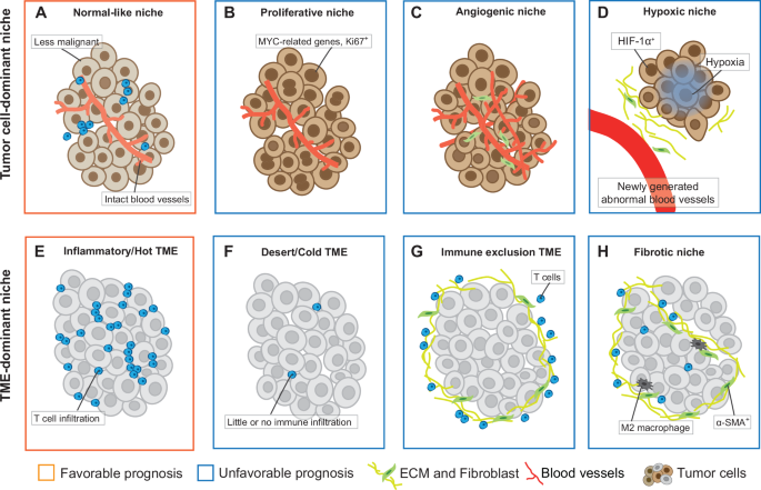
A Normal-like niche. B Proliferative niche. C Angiogenic niche. D Hypoxic niche. E Inflammatory TME. F Desert TME. G Immune exclusion TME. H Fibrotic niche. TME, tumor microenvironment.

Full size image

For spatial studies of nonparenchymal cells, CAF and T cells are among the most important types (Fig. 2E–H). In non-small cell lung cancer, IMC data have identified 11 spatially distinct CAF phenotypes, each associated with different prognostic patient groups¹⁵⁶. In breast cancer, the stromal niche is associated with tumor phenotype, but only one poorly cohesive stromal niche, containing proliferative vimentin-producing fibroblasts, is independently associated with poor disease-free and overall survival (Fig. 2H)¹⁵⁷. As for immune phenotypes, the inflamed, altered, and desert phenotype are directly defined by the spatial distribution of CD8⁺ T cells (Fig. 2E, F and G)^73,158. Among them, the inflamed phenotype of patients with non-small cell lung cancer is an independent prognostic factor for disease-specific survival and recurrence time¹⁵⁸ (Fig. 2E)

Furthermore, some CNs composed of multiple cells co-localized with T cells have also been shown to shape anti-tumor immunity and could predict better clinical behavior, such as pan-immune CNs, T cell infiltration CNs and lymphoid-enriched CNs^95,157. In contrast, a microenvironmental community characterized by vascularization with T cell involvement is associated with increased risk of death⁹⁵. In addition to T cells, CNs composed of other immune cells also affect prognosis. For instance, CNs composed of M1-like MDMs, neutrophils, and M1-like microglia, is associated with increased survival in patients with high-grade glioma¹⁰⁸, although the frequency of M1-like MDMs is not associated with OS, highlighting the importance of spatial structure¹⁰⁸. However, the relationship between these CNs and survival is not uniform and may need to be explored separately in different histological subtypes. For example, in patients with lung adenocarcinoma, lymphoid-enriched CNs are less in the lepidic tumors with a good prognosis, but more common in the solid tumor subtype. In another acinar tumor, more B-cell-enriched CNs indicate better survival⁹⁵.

Spatial biomarkers of immunotherapy

Although previous omics studies have found many biomarkers of immunotherapy, such as mutation burden and PD-L1 expression, spatial measurements further reveal spatial biomarkers that predict therapeutic efficacy and explain the mechanism of immune escape. For example, multiplex immunohistochemistry (mIHC) or multiplex immunofluorescence (mIF) indicates response prediction for immunotherapy by measuring CD8⁺ cell density within intratumoral/peritumoral compartments or co-expression markers indicative of T cell activation¹⁵⁹. CODEX further quantify finer spatial distributions of cell subtypes with more proteins. For example, in patients with cutaneous T-cell lymphoma treated with pembrolizumab, the spatial distribution of effector PD-1⁺ CD4⁺ T cells and immunosuppressive Tregs differs between responders and non-responders¹⁶⁰.

Meanwhile, the spatial relationship between immune cells and cancer cells is also related to the response to immunotherapy. The proximity of PD-1 on T cells to PD-L1 on tumor cells can be measured by mIHC or mIF, which has potential advantages over tumor mutational burden or PD-L1 expression¹⁵⁹. Similarly, the proportion of proliferating CD8⁺ TCF1⁺ T cells and MHC II⁺ cancer cells are the dominant predictor of treatment response in a randomized neoadjuvant immune checkpoint blockade trial for TNBC, followed by spatial interactions between cancer cells-B cells and cancer cells-granzyme B⁺ T cells¹⁶¹. In melanoma patients who underwent adoptive cell therapy with ex vivo expanded autologous TILs, more interactions between CD8⁺ or CD8⁺ PD-1⁺ TILs and CD11c⁺ cells are observed within tumor islets and stromal regions in responding patients compared with non-responders¹⁶². In advanced RCC patients, the spatial co-expression of the ligand-receptor pair COL4A1 and ITGAV is significantly increased after immunotherapy compared with immunotherapy naïve tumors, helping to elucidate the mechanisms of immune response¹⁶³.

Multicellular spatial organization also provides additional insights into immunotherapy. TLS is a promising predictive biomarker associated with response to immune therapies, as it forms discrete TME that provide sites for antigen presentation and cytokine-mediated signaling (Fig. 1B)^{93,164,165,166}. In RCC, characterization of distinct TLSs suggests that TLS-positive tumors exhibit a high frequency of IgG-producing plasma cells and are associated with improved outcomes with immune therapy¹⁶⁷. Additionally, some newly defined immune phenotypes such as “inflamed”^20,21 or “immunity hub”¹⁶⁸, are also strongly associated with therapy response. In TNBC, whole-slide staining for CD8 defines three spatial immunophenotypes: inflamed phenotype has the best prognosis, excluded phenotypes intermediate and the ignored phenotypes have the worst prognosis²¹. Further transcriptome analyses demonstrates that these immunophenotypes are characterized by different modes of T cell immune-evasion²¹.

In summary, spatial signatures have optimized previous biomarkers for predicting therapeutic efficacy, and continued spatial analysis that preserves tissue’s microanatomical structure holds promise to improve response prediction factors and provide deeper insights into the mechanisms of response.

While spatial profiling techniques have provided novel insights, several challenges remain for the field (Fig. 3).

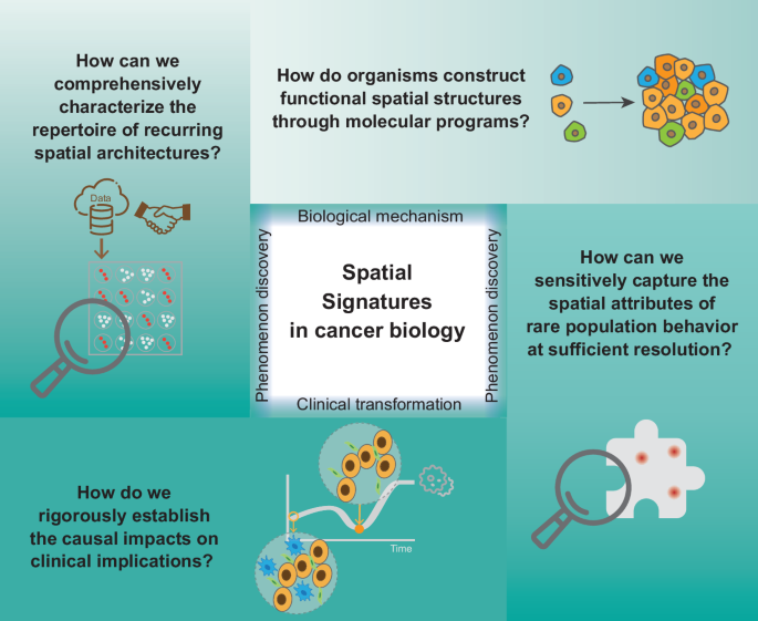
Key challenges in studying spatial signatures in cancer biology.

Full size image

First, the molecular mechanisms of spatial organization have not yet been fully revealed. The spatial characteristics of biological tissue structures often reflect their intrinsic molecular biological processes, especially some recurring spatial organizations. This is mainly because it is difficult to fully capture the spatial changes of different biological molecules (such as transcripts, proteins, phosphorylated proteins, metabolites, etc.) due to sensitivity limitations. Fortunately, emerging multi-omics spatial analysis technologies have realized joint profiling of the epigenome and transcriptome by co-sequencing chromatin accessibility and gene expression, or histone modifications to provide multimodal data to reveal spatial regulatory mechanisms^169,170. In addition, computational methods for spatial pseudo-time have also made certain progress, allowing researchers to infer dynamic molecular processes from spatial profiles at a single time point^132,171. Further, in order to verify the causal relationship, high-throughput perturbation experiments¹⁷² and computer virtual perturbation¹⁷³ become powerful tools¹⁷⁴. In the future, unbiased genome-wide joint determination of epigenome and transcriptome on the same tissue section at the single-cell resolution needs to be achieved, and FFPE samples may be better utilized. At the same time, given the obvious heterogeneity in the spatial organization of different biological systems, computational tools that can comprehensively analyze complex patterns in spatial data still need to be developed in the future. In addition, intratumor heterogeneity may affect the validity of tissue microarrays (TMAs)¹⁷⁵. Some studies suggest that, in most cases, two 0.6 mm tissue cores are sufficient to represent the staining observed in the entire tissue section^176,177,178. However, TMAs should still be used with caution for certain biomarkers with location-dependent expression, such as hypoxia markers^179,180,181. A potential solution is to conduct large TMA studies to reduce sampling error by increasing the cohort size or to use heterogeneous markers, such as the proliferation marker Ki-67 or tumor microvessel density, to examine intratumor heterogeneity¹⁷⁸.

Second, some recurrent tissue motifs across multiple datasets or common patterns of spatial signatures have not been fully revealed. Although the mechanisms and processes of disease occurrence may vary from individual to individual, there are certain commonalities in the spatial arrangement of key cell types and communities in tissues. This shift from individualization to groupization is of great significance for our understanding of the complexity of biological systems. However, due to the cost of spatial technology, most spatial analyses are still focused on specific samples, mainly reflecting the characteristics of tissue structure in specific situations. At the same time, data may show obvious batch effects¹⁸², which refers to technical biases. These factors have the potential to obscure genuine biological signals, thereby complicating data interpretation and integration. Currently, there are some methods that integrate multiple datasets (e.g., SCGP-Extension¹⁸³ and STAligner¹⁸⁴). Most integration methods are originally designed to learn embeddings across multiple slices, and it is still difficult to determine which tool has the best overall clustering performance among all pairs after integration¹⁴⁰. Using TMAs can alleviate the cost and batch issues to some extent. One of the benefits is the availability of FFPE archival tissues, and inter-batch variability is reduced by analyzing all samples simultaneously. This approach is important for quality assurance and is cost-effective in large cohort experiments¹⁷⁸. In the future, more project cooperations and data disclosure need to be advocated to support the establishment of tissue spatial data atlas. At the same time, more powerful integration tools are still needed in the future. They need to show good scalability for large datasets, merge data from various sources or conditions (e.g., different anatomic regions or development stages), enhance data robustness and reveal common patterns that are not apparent in an individual dataset¹⁴⁰.

Third, it remains difficult to comprehensively analyze rare cell populations. For spatial omics technologies with limited resolution, the locations of rare cells are inferred by deconvolution algorithms or scoring of signature genes, but the results often contain a large amount of noise. Although more and more single-cell level spatial technologies are emerging, they can only capture dozens to hundreds of molecules per cell and may not cover the interesting rare cell type. In cases with limited prior knowledge of rare cell type, researchers may need to prioritize whole-slide capture as a primary approach, since the core region of the TMA may not sufficiently capture these cells, potentially compromising the characterization of statistical effects and spatial distribution. In future, advanced spatial omics techniques and matching algorithms may be able to better mine rare cell subtypes.

A fourth challenge is that the relationships between spatial features and underlying biological functions or clinical implications remain unclear. A large number of studies have found that different cell communities or spatial distribution characteristics in tumor tissues are significantly correlated with clinical prognosis, indicating that spatial features may have an important impact on the occurrence and development of tumors. However, the causal relationship between spatial features and tumor biology has not been accurately determined. In the future, the spatial characteristics found by different computational methods need further verification, which requires more benchmarking researches on different approaches. And larger sample cohorts can also help discover new clinically significant associations by improving statistical power. Dynamic time series and perturbation experiments to track changes in spatial features during tumor progression are also possible ways to solve this problem. By artificially regulating the impact of these features on tumor, the causal relationship between them can be more clearly determined.

In summary, this review comprehensively summarizes the recent advances in the study of spatial signatures. By leveraging computational methods, these spatially resolved molecular and cellular signatures characterized across multiple scales have revealed unprecedented insights into TME.