Quantum error mitigation in quantum annealing

Introduction
Quantum computation has emerged as a computational paradigm with the potential to solve complex problems that remain beyond the capabilities of classical computers. However, its performance is substantially hampered by environmental noise and hardware imperfections. Quantum error correction (QEC)1,2 is regarded as the ultimate solution to eliminating the impact of these errors, but the significant overhead of QEC limits its practicality to very large scales, far beyond the current state of technology3. Recently, quantum error mitigation (QEM) has been proposed4,5,6,7 as a near-term solution that can be used to estimate error-free expectation values when the impact of noise is small. Among the various QEM techniques, zero-noise extrapolation (ZNE)4,5 stands out as one of the most practical methods. In ZNE, one systematically varies the noise amplitude experienced by the system. By observing the system’s response to this controlled change, it becomes possible to make predictions about how the system would behave under noise-free conditions.
While QEM was initially developed and tested for circuit-model quantum computing8,9,10,11,12, the same principles can be applied to other quantum-computing protocols, including quantum annealing (QA)13. Over the past few years, quantum simulation has evolved into an important application of QA for the exploration of exotic states of condensed matter systems14,15,16,17 and their quantum phase transitions18,19,20. QEM can enhance the accuracy of expectation values in quantum simulation experiments without incurring any additional overhead in qubit count, in contrast to previous quantum-annealing correction techniques21,22,23,24,25,26,27,28,29,30,31,32. Indeed, the first experimental attempt to extract information about noise-free evolution via extrapolation was reported in ref. 33, in which QA performance was examined as a function of temperature for a problem with a very small spectral gap. By extrapolating the final ground state probability to zero temperature, the noise-free Landau-Zener behavior was replicated (see 3 and 4 of ref. 33). Recently, a few error-mitigation proposals for QA or adiabatic quantum computation have emerged34,35,36. However, they remain largely theoretical with no relevance to the existing quantum-annealing processors.
In this paper, we introduce practical ZNE techniques for QA. We provide a theoretical description with a particular emphasis on extracting information about quantum phase transitions and post-critical dynamics. We then employ ZNE in experimental investigations into the dynamics of a 1D quantum Ising spin chain. The extrapolated results compare well with exact solutions as well as time-dependent density matrix renormalization group (DMRG) simulations for the closed system Schrödinger evolution across a wide range of control parameters. We investigate kink density and kink correlations. While kink density is well described by the Kibble-Zurek mechanism, with experimental error primarily influenced by thermal noise, kink correlations are more sensitive to post-critical dynamics and non-thermal errors.
Results
Zero-noise extrapolation in annealers
The Hamiltonian of an annealing-based quantum processing unit (QPU) is written as
where the problem Hamiltonian is
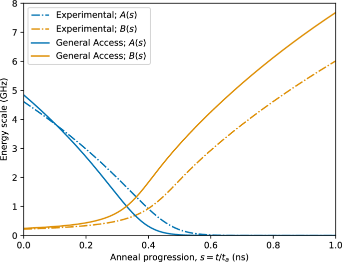
and s = t/ta, with t being time and ta being the annealing time. The energy scales Γ(s) and ({mathcal{J}}(s)) evolve with time in such a way that (Gamma (0),gg, {mathcal{J}}(0)) and (Gamma (1),ll, {mathcal{J}}(1)). They are predetermined at the time of calibration (see Fig. 6 in “Methods—Critical and post-critical dynamics of the transverse field Ising chain”). The dimensionless biases (hi) and coupling coefficients (Jij) are programmable.
To incorporate all sources of error, whether thermal, 1/f noise, or parameter misspecification, we consider the qubits to be in contact with their environment. The total Hamiltonian is written as
where HB is the environment Hamiltonian, and
describes the interaction between system and environment. The operators Qα act on the corresponding environments, with α spanning all sources of noise. The operators ({{mathcal{O}}}^{alpha }) are local unitless operators acting on the qubits, typically realized as Pauli matrices (e.g., ({sigma }_{i}^{z}) for flux noise and ({sigma }_{i}^{y}) for charge noise). We can accommodate static control (miscalibration) errors within the same framework by taking Qα to be a constant random value. For example, to incorporate static errors δhi (δJij) in the Hamiltonian parameters, we use ({{mathcal{O}}}^{alpha }={sigma }_{i}^{z},({mathrm{or}}; {sigma }_{i}^{z}{sigma }_{j}^{z})) and (sqrt{gamma }{Q}^{alpha }/{mathcal{J}}(s)=delta {h}_{i},(or; delta {J}_{ij})). The corresponding noise spectral density in that case is a δ-function at zero frequency. The prefactor (sqrt{gamma }) is introduced to keep track of the perturbation order; γ can be thought of as an overall decay rate, in units of Hz, multiplying all relaxation and dephasing rates. Its precise definition is unimportant for our discussion.
The state of an open quantum system is commonly described by the reduced density matrix ρ(t), which is the solution to a master equation, e.g., Bloch-Redfield37 or Lindblad38,39. As we show in “Methods—Open quantum model”, the density matrix at the end of the evolution can be expanded in powers of γ as
where ρ0(ta) is the noise-free contribution to the density matrix and ρμ>0(ta) take care of perturbative corrections due to the environment. As such, any observable A at the end of annealing can be expanded as
where
The zeroth order term, ({langle A({t}_{a})rangle }_{0}), is the error-free expectation value for coherent evolution. Our goal is to extract ({langle A({t}_{a})rangle }_{0}) by extrapolation from a set of noisy evolutions.
ZNE is implemented by amplifying the effect of noise by a controllable factor λ in such a way that ρ0(ta) and therefore ({langle A({t}_{a})rangle }_{0}) remain unchanged. This can be easily achieved in theory by increasing the coupling coefficient:
Substituting (8) into (7) and (6), and expanding up to order M, we obtain
where ({C}_{mu }={langle A({t}_{a})rangle }_{mu }). We can now estimate the error-free expectation value, ({langle A({t}_{a})rangle }_{0}={C}_{0}), by measuring 〈A(ta, λ)〉 for a range of λ-values, fitting the result into (9), and extrapolating back to λ → 0. When the effect of the environment is small, only a few terms in the expansion (usually M = 1 or 2) suffice to yield a good estimate. Terms in these series can be bounded and evaluated in principle as a function of a noise model (see “Methods—Open quantum model”) and target statistic. As noted later, we are able to identify C1 as zero in one experiment and work with a pure quadratic form, but more generally we justify the perturbative approach experimentally.
Since continuous dynamics can be modeled as a discrete process with Trotterization, many existing results can be applied to annealing after appropriate accommodation of a continuous limit4,5. In practice, it is not feasible to amplify noise by increasing γ because it requires manipulating the qubits’ environment at the microscopic level. However, it is possible to mimic such an effect by practical means: temperature rescaling and problem-Hamiltonian rescaling. We discuss temperature rescaling with experimental verification in the section “Zero-temperature extrapolation”. We present a new problem-Hamiltonian rescaling motivated by an understanding of critical phenomena, and verified experimentally in section “Zero-time extrapolation”. Experimental implementation details are presented in “Methods—Experimental details”, including code examples sufficient for the reproduction of results on generally-accessible (GA) QPUs. These QPUs are accessible via the LeapTM quantum cloud service. The validity and limitations of a critical-phenomena-based error-correction methodology are thoroughly explored for the 1D model in “Methods—Critical and post-critical dynamics of the transverse field Ising chain”. We compare to exact DMRG and Buguliobov-de Gennes simulations, described in “Methods—Simulation of dynamics”.
Zero-temperature extrapolation
The simplest way to increase the influence of a thermal environment is by increasing its temperature T. Clearly, the coherent contribution to the density matrix ρ0(ta) remains unaffected by changing T. As we show in “Methods—Open quantum model”, in the regime of weak coupling to the environment, all decay processes, including relaxation and dephasing, are functions of the thermal noise spectral density, which we denote by S(ω) (in general, different qubits may be coupled to different heat baths with different spectral densities, but these details don’t affect our argument. See “Methods—Open quantum model” for more details)40. We stress that experimentally attainable annealing times are away from the regime of fast quenches, where deviations from Kibble-Zurek mechanism have been predicted in ref. 41. For example, the relaxation rate between states (leftvert nrightrangle) and (leftvert mrightrangle) is proportional to S(ωnm), where ωnm = En − Em is the energy difference between the two states, and the dephasing rates are functions of S(0) or spectral density at low frequencies. For an environment in thermal equilibrium at temperature T, the noise spectral density can be expressed as (ℏ = kB = 1)
where ζ(ω) is an antisymmetric function. High-frequency components of the environment (ω ≫ T) follow adiabatically the slow evolution of the system and therefore do not induce transitions amongst system states. In our experimental regime (ℏ/ta ≪ kBT), only transitions between states for which ωnm ≲ T affect the density matrix. We can, therefore, expand e−ω/T in the denominator to first order to obtain S(ω) ≈ Tζ(ω)/ω. This means that
Since the coefficient λ multiplies all decay rates, it can be factored out and absorbed into the coupling coefficient γ, leading to (8). Factoring out λ would keep ρμ(ta) unchanged in (5), resulting in expansion (9), thus allowing ZNE.
While the above explanation relied on low energy expansion of the noise spectral density, the conclusion goes beyond that. As long as the change in T can be treated as a perturbation, an expansion similar to (9) is expected, but with different coefficients Cμ and with C0 representing the zero-temperature expectation value, which is not necessarily equivalent to the error-free one (see below).
We experimentally tested zero-T extrapolation using a D-Wave Advantage2TM prototype processor, with 232 flux qubits coupled in a one-dimensional periodic chain. Note that GA QPUs do not currently allow for manipulation of temperature. We applied zero bias hi = 0 to all qubits and used uniform ferromagnetic coupling Jij = −1.8. We annealed the QPU using the fast-anneal protocol to simulate the critical dynamics of a transverse-field Ising spin chain. Details of the experiment are provided in “Methods—Experimental details” and ref. 18.
We measured kink density, defined as
where L is the length of the chain and
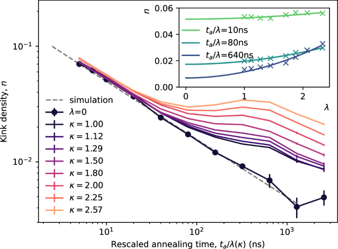
is the kink number operator. Note that energy is a linear function of the kink density, and also that correlation length (xi =frac{1}{n}). Data was collected at four temperatures and for a range of annealing time, as shown in Fig. 1, alongside the linearly extrapolated (ZNE) prediction. Experimental data follows simulation, well described by Kibble-Zurek theory (a power law, section “Critical and post-critical dynamics of the transverse field Ising chain”), at small ta and then deviates upwards. ZNE produces improved agreement on longer time scales. A deviation upwards is apparent on longer time scales, where we infer that the perturbative approach is no longer successful—it is also more challenging to analyze the regime of small kink density owing to reduced statistics and finite-size effects. The inset shows examples of the linear extrapolation as a function of temperature.

Kink density is plotted as a function of annealing time for four different temperatures. A T-dependent deviation from the simulation is due primarily to thermal excitations. The darkest line marked by circles is the ZNE extrapolation result, determined by linear extrapolation at each ta; examples of the linear extrapolation at several ta are shown in the inset. Data is in good agreement with the simulation result on short time scales, and ZNE allows improved agreement on longer time scales. Simulation is also in good agreement with the Kibble-Zurek mechanism (power-law) from Eqn (79) through the experimental parameter range, where τQ = 0.52ta at J = −1.8.
While zero-T extrapolation seems to reproduce correct results for the kink density, it is not expected to correct miscalibration or other non-thermal errors that do not depend on T. These errors can affect other physical observables such as higher-order correlations, as we shall discuss later. Moreover, temperature control is not a generally accessible feature for D-WaveTM QPUs, which, therefore do not generally support ZNE in T; methods requiring only generally available controls are preferable.
Zero-time extrapolation
A more desirable way of amplifying noise is via energy-time rescaling. Since γ is multiplied by ta in (5), it is possible to mimic the effect of increasing γ by increasing ta. However, in order to keep the noiseless unitary evolution ρ0(ta) unaffected, one needs to rescale both anneal time and energy. This can be achieved by substituting ta → λta and HS → HS/λ, which leaves ({int}^{{t}_{a}}{H}_{S}(t)dt), and therefore the unitary time evolution operator, unchanged. In gate-model quantum computation, this approach is referred to as analog-ZNE4, in contrast to digital-ZNE, in which noise is amplified by inserting additional (identity) gates12. Intuitively, extending the annealing time would increase the effect of relaxation and dephasing on the qubits. Reducing the energy scale, on the other hand, would amplify the relative impact of control errors, provided that these errors are not altered by the rescaling. These all lead to a λ-dependent reduction of accuracy. It should be noted that ρμ>0(ta) may also have some residual dependence on λ, but that can be easily incorporated into the Taylor expansion (9) by redefining the expansion coefficients Cμ. This means that only the invariance of ρ0(ta) is required for ZNE to work.
In annealing QPUs, rescaling the system Hamiltonian HS in (1) is challenging because both Γ(s) and ({mathcal{J}}(s)) are not programmable. However, one can easily scale down the problem Hamiltonian HP by reprogramming hi and Jij in (2). Since only one part of HS is being rescaled, ensuring that the coherent evolution remains unaffected is nontrivial. Let us introduce a problem-Hamiltonian rescaling as
We need to choose κ(λ) in such a way that ρ0(ta) becomes independent of λ. In general, this may not be exactly possible, but can be achieved approximately. In particular, when the statistic of interest is dominated by dynamics within a narrow region in s, one can obtain an approximate κ(λ) in such a way that the coherent dynamics remain unaffected by the rescaling (see “Methods—‘Practical energy-time rescaling’ and ‘Experimental details’ ” for details). This is the case for quantum phase transition, where critical dynamics occur within a narrow region close to the critical point sc, and some statistics only depend on the speed of passing this point. Rescaling HP would move the critical point to a new point ({s}_{c}^{kappa }) with a new effective speed. This change has to be compensated by rescaling the annealing time as shown in “Methods—Practical energy-time rescaling”. For the case of a 1D chain with full-scale problem Hamiltonian ({H}_{P}=-sum {sigma }_{i}^{z}{sigma }_{i+1}^{z}) the critical point ({s}_{c}^{kappa }) for the rescaled Hamiltonian is the solution to (Gamma ({s}_{c}^{kappa })={mathcal{J}}({s}_{c}^{kappa })/kappa). We therefore obtain (see “Methods—Practical energy-time rescaling”)
Processor-wide control of the anneal rate through the critical region(s), and determination of the energy scales, is challenging in large-scale general-purpose QPUs. An alternative empirical method for the determination of λ is described in “Methods—Experimental details—Experimental Advantage2 prototype methodology at a scale L = 232”, with qualitatively matched results. Once κ(λ) is determined, we can use (9) to fit the data and extrapolate to λ → 0.
We can first consider extrapolation of the kink density. We used the GA Advantage2 prototype Advantage2_prototype2.3. Code required to reproduce the experiment is described in “Methods—Experimental details—GA Advantage2 prototype methodology at a scale L = 1024”. For a thermal environment at temperature T, scaling up the Hamiltonian is equivalent to scaling down the temperature, i.e., T → κ(λ)T ~ λT, where in the last step we expanded κ(λ) to linear order. As we discussed in the previous section, this can be effectively modeled by γ → λγ. Since we also scale ta → λta, to the leading order in λ, the expansion coefficients in (5) scale as
Therefore, for thermal noise, leading dependence on λ in Taylor expansions is of second order:
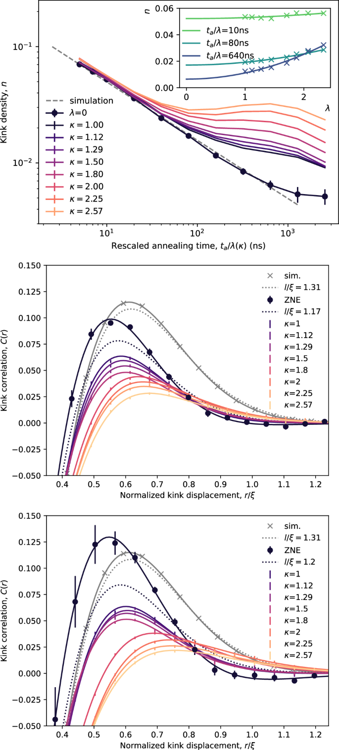
Extrapolation for kink-density using (15) and (17) are shown in Fig. 2, with results qualitatively similar to Fig. 1. The collapse of the kink density at small ta indicates decoupling from thermal noise, so extrapolation in this coherent regime has little impact on statistics. For longer annealing times, the extrapolation improves agreement with the simulation result, in close alignment with the Kibble-Zurek mechanism (power-law) throughout the experimental range. Variations on the methodology are explored in methods with similar results down to the regime of small kink densities (≪10−2) where extrapolation becomes challenging.
For the GA Advantage2 prototype solver, the kink density is calculated for various coupling strengths (Jij = −1.8/κ) with time rescaled by λ(κ) assuming the published schedule and (15). Agreement is reasonable for small values of ta/λ (larger energy, shorter time), but deviate on longer time scales. Quadratic extrapolation to λ(κ) = 0 (examples shown inset) improves the agreement with simulation on longer time scales.
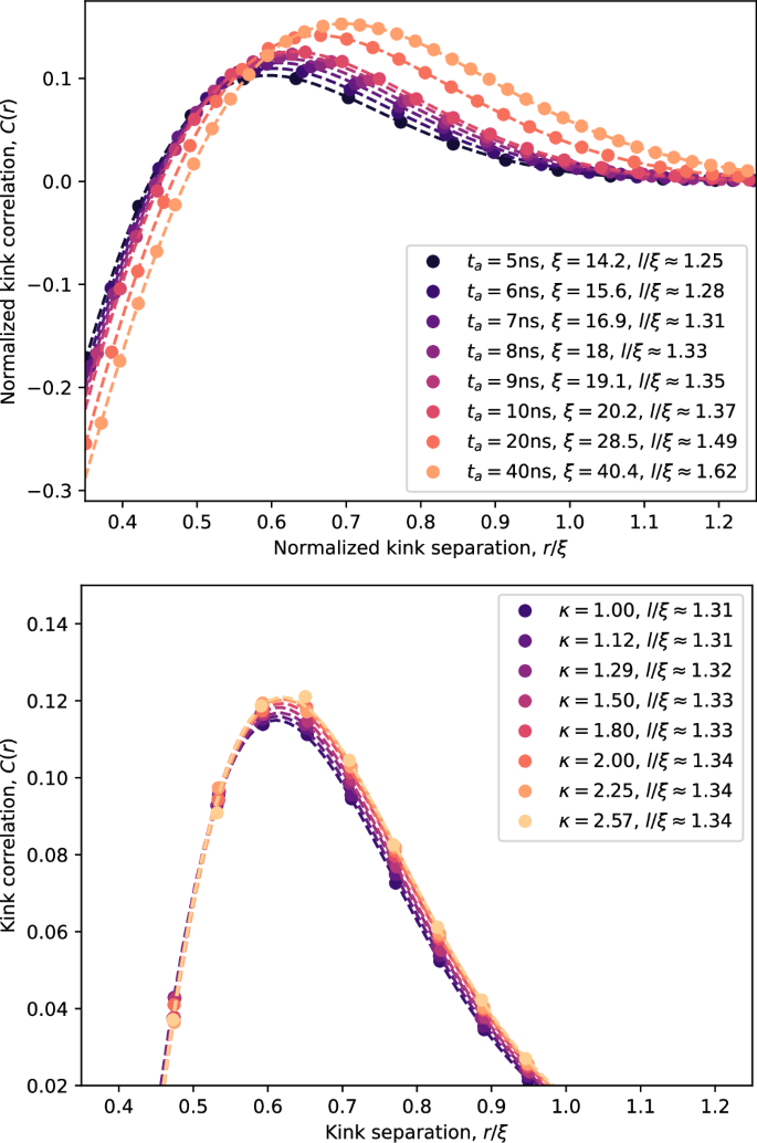
While kink density is only sensitive to thermal noise, non-thermal and post-critical dynamics are expected to impact the accuracy of other statistics. In Fig. 3, we show the kink correlation defined by
Experimental data shows a significant deviation from exact simulations with the peak being suppressed. This deviation was first observed in ref. 18 and attributed to disorder caused by control errors and 1/f noise. Disorder in the potential energy can draw kinks toward local minima, thereby affecting their correlation while leaving their density unchanged. ZNE increases the peak height, bringing it closer to the exact simulation (the fit to the extrapolated points corresponds to a four-parameter function, see “Methods—Experimental details”). However, a discrepancy still persists, which we attribute to post-critical dynamics. After the critical point, kinks are expected to continue moving, while their total number (or density) remains unchanged. Consequently, the position and size of the kink correlation peak would shift due to the energy-time rescaling, even in the absence of noise. In other words, not all the observed changes are noise-related, and thus cannot all be corrected by ZNE.
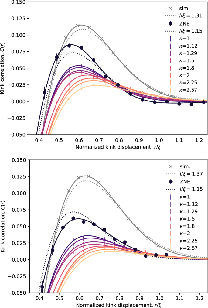
Kink correlations (18) are shown for experiments performed at 7ns (top) and 10ns (bottom) for κ = 1, alongside experiments at other κ with λ(κ) rescaled according to (15). Simulation results are also shown. All experiments show a peak value in C(r), consistent with a combination of critical and coherent post-critical dynamics. The ZNE curve is shifted to the left of the simulation result, and curve height is suppressed at increased κ (reduced energy scale and increased simulation time). The enhancement of the peak height, towards the simulation result by ZNE is a demonstration of error mitigation. At 7ns both simulation and extrapolated data are well described by a 1-parameter theory, but curves differ in l/ξ; simulation is consistent with enhanced post-critical dynamics (larger l/ξ). At 10ns (and more generally with increasing ta) the curve height is suppressed relative to simulation and theory, which we attribute to accumulation of errors beyond the regime correctable perturbatively.
This phenomenon is discussed in detail in “Methods—Critical and post-critical dynamics of the transverse field Ising chain” (see also refs. 42,43), where an approximate analytical solution with an additional length scale l is introduced. In the absence of post-critical dynamics, we expect l = ξ. As the dynamics continue after the critical point, l increases due to quasiparticle phase-scrambling (see “Methods—Critical and post-critical dynamics of the transverse field Ising chain”). This allows us to control the influence of post-critical dynamics by varying l at fixed kink density (1/ξ). For the case of D-Wave’s annealing schedule, as κ → 0 (in ZNE), we expect l/ξ → 1, which may differ from the corresponding value in the exact simulation at κ = 1. Figure 3 shows the kink correlation for two values of l/ξ used to fit both the exact simulation and the extrapolated curves. As expected, the extrapolated curve corresponds to a smaller l/ξ compared to the exact simulation. Increasing the annealing time ta from 7 ns (top panel) to 10 ns (bottom panel), raises the peak height in the exact simulation, and thereby the corresponding l/ξ, consistent with the extended post-critical dynamics. For ZNE, however, the peak height decreases; the discrepancy may be attributed to unmitigated systematic errors in the Hamiltonian parameters (see “Methods”).
Discussion
We have demonstrated the successful implementation of zero-noise extrapolation (ZNE) for quantum annealing. We presented an efficient problem-Hamiltonian rescaling methodology and a temperature rescaling method, both applied to Advantage2 prototypes. Through the analysis of critical dynamics in a 1D quantum spin chain, we mitigated the impact of thermal noise on kink density, extending the time-scales on which agreement with theory is possible. Additionally, we mitigated the influence of non-thermal errors, as evidenced by the estimation of kink correlations. Extrapolated results show improved agreement with Bogoliubov-de Gennes and DMRG simulation results.
Our problem-Hamiltonian rescaling methodology was developed assuming the annealing schedule can be linearized about some particular s. Whilst this works well for kink density, other statistics such as the kink correlations are shown to be sensitive to post-critical dynamics, and a theory is developed for this. Problem-Hamiltonian rescaling is understood to mitigate for noise, but can distort the contribution of post-critical dynamics to statistics, so care is required.
It is important to emphasize that ZNE enhances the accuracy of expectation values, but does not directly provide higher-quality samples. Nevertheless, sample or subspace frequencies, where measurable, can be extrapolated to obtain insight into statistics such as time-to-solution44 for increasingly lower noise and more coherent systems. This provides a performance model for the QPU, and can quantify coherence and noise levels requirements. When the objective involves optimizing for a lower energy solution, quantum-annealing correction techniques21,22,23,24,25,26,27,28,29,30,31,32 may represent a more appropriate approach to enhance overall performance. The technique described in this work can be applied to tackle more intricate challenges, such as quantum simulations of exotic magnetic materials. Leveraging ZNE makes it feasible to estimate expectation values in situations where classical computation approaches become intractable.
Methods
Open quantum model
In this appendix, we use open quantum modeling to explain ZNE. We write the total Hamiltonian as
where HS and HB are system and bath Hamiltonians, respectively. We write the interaction Hamiltonian in a general form as
where ({{mathcal{O}}}^{alpha }) is an operator acting on the system and Qα is the noise operator acting on the corresponding environment. The operators ({{mathcal{O}}}^{alpha }) are typically Pauli matrices, e.g., ({sigma }_{alpha }^{z}) for flux noise and ({sigma }_{alpha }^{y}) for charge noise. For static noise, such as control error, Qα can be considered as a constant random energy.
In open quantum systems, the state of the system is described by the reduced density matrix ρ(t). We choose the preferred basis to be the eigenstates (leftvert nrightrangle) of the system Hamiltonian HS with eigenvalues En. The Bloch-Redfield equation for the reduced density matrix ρ(t) is written as37
where ωnm = En − Em and the Redfield tensor is defined as
with
Here, ({{mathcal{O}}}_{nm}^{alpha }equiv leftlangle nrightvert {{mathcal{O}}}^{alpha }leftvert mrightrangle) and the noise spectral density is defined as
For the case of uncorrelated heat baths we have
For a time-dependent system Hamiltonian, the generalized Bloch-Redfield equation becomes45
where
In the energy basis, we write the density matrix as a linear vector with 22N elements:
The master equation becomes a matrix equation:
where
is a diagonal matrix made of energy differences and (hat{M}) and (hat{R}) are the basis-rotation and relaxation matrices corresponding to Mnmkl and Rnmkl, respectively. A formal solution to this equation is
The time-ordering operator ({mathcal{T}}) is introduced to take care of non-commuting (hat{gamma }(t)), (hat{M}(t)), and (hat{R}(t)) at different times. Changing the integration variable to s = τ/ta, we get
The term (gamma hat{R}(s)) in the exponent takes care of all relaxation and dephasing processes during the evolution, with γ appearing as a common factor in all time-scales. In the limit of small γ when those decay processes are not very strong, it is possible to assume this term is small and expand the exponent. Using Taylor expansion, we can write
where
is the noise-free contribution to the density matrix and
captures the effect of noise to order μ in perturbation. Turning back the density matrices from vector form to matrix form we obtain (5).
In some cases, only a small number of energy states get occupied during the annealing process. Therefore, we only need to incorporate relaxation and dephasing processes between those states. The experiment reported in ref. 33 is one such case. The evolution is limited to the lowest two energy states, during which the relaxation process is extremely slow. This allows expansion in powers of those relaxation rates only, although other decay processes could be much faster. As a result zero-T extrapolation worked for time scales millions of times longer than the expected single-qubit decoherence time of the qubits.
Practical energy-time rescaling
The goal of this section is to introduce a relation between energy and time rescaling so that the critical dynamics remain unchanged. We first write the time-dependent Hamiltonian in a dimensionless form with one dimensionless parameter τQ, which measures the speed of passing the critical point. The same quantity is used in some theory papers (see e.g., refs. 42,43) and rederived in “Methods—Critical and post-critical dynamics of the transverse field Ising chain”, hence our formalism allows direct comparison with these analytical results.
We start by writing the Hamiltonian (1) as
where
is the dimensionless transverse field. The corresponding Schrödinger equation reads
Introducing a dimensionless time
we can write (39) in dimensionless form
where
is the dimensionless Hamiltonian. Note that (tilde{t}in [0,{tilde{t}}_{a}]) with ({tilde{t}}_{a}={t}_{a}mathop{int}nolimits_{0}^{1}{mathcal{J}}(s)ds) being the dimensionless annealing time.
For fast annealing, only the speed of passing the critical point determines the critical dynamics. We define the critical point s = sc by
where gc is the critical value of g. Using linear expansion near the critical point we write
where τQ is the dimensionless quench time scale and ({tilde{t}}_{c}=tilde{t}({s}_{c})). It is possible to express Kibble-Zurek dynamics only in terms of τQ. In other words, two systems with the same τQ are expected to yield the same statistics as long as only critical dynamics affect their evolution. For a slower evolution where the dynamics outside the critical region affect the results, details of the schedule become important.
We expand the schedule near the critical point as
where Γc ≡ Γ(sc), ({Gamma }_{c}^{{prime} }equiv {[{partial }_{s}Gamma (s)]}_{s = {s}_{c}}), etc. Expanding g(s) near sc, we obtain
On the other hand
Therefore,
Comparing with (44), we obtain
where
defines a time scale that only depends on the annealing schedule. For a 1D spin chain with a problem Hamiltonian
the critical point is the point where ({Gamma }_{c}={mathcal{J}}({s}_{c})), thus gc = 1. On the other hand, for 2D and 3D problems we have gc > 1 and, therefore, we expect the critical point to occur earlier in the schedule.
In order for the two systems to have the same critical dynamics, they need to have the same τQ. Equation (50) requires that ta should be scaled the same way as tQ in (51). If both Γ(s) and ({mathcal{J}}(s)) are scaled the same way such that HS → HS/κ, we obtain tQ → κtQ, therefore we need λ = κ, as expected for simple rescaling.
For the more practical case of only rescaling HP, it is equivalent to ({mathcal{J}}(s)to {mathcal{J}}(s)/kappa) without changing Γ(s). Obviously, the critical point will be shifted to a new point ({s}_{c}^{kappa }) which is the solution to (Gamma ({s}_{c}^{kappa })={g}_{c}{mathcal{J}}({s}_{c}^{kappa })/kappa). Thus, one needs to calculate the new ({t}_{Q}^{kappa }), obtained from (51) at ({s}_{c}^{kappa }). The correct time rescaling coefficient will therefore be:
For the case of the 1D transverse field Ising problem, we can write
where ({Gamma }_{c}^{kappa {prime} }={Gamma }^{{prime} }({s}_{c}^{kappa })), etc. We should emphasize that the above analysis is based on the assumption that Kibble-Zurek dynamics can be completely characterized by a single time-scale. In reality, there are other time scales that are relevant to post-critical dynamics, which may explain the small ta-dependence in Fig. 8a.
Critical and post-critical dynamics of the transverse field Ising chain
Quantum Ising chain
The transverse field quantum Ising chain is46
where we assume periodic boundary conditions, ({overrightarrow{sigma }}_{N+1},=,{overrightarrow{sigma }}_{1}), and even N for definiteness. For N → ∞ the quantum critical point at ({Gamma }_{c}/{{mathcal{J}}}_{c}=1) separates the paramagnetic and ferromagnetic phases. Note that the programmed ferromagnetic coupling (Jij = −1.8/κ) is absorbed into the definition of ({mathcal{J}}) for purposes of this section. After the Jordan-Wigner transformation:
introducing fermionic annihilation operators cn, the Hamiltonian (55) becomes
Here the projectors
define subspaces with even/odd numbers of fermions as the parity, related to ({prod }_{n}{sigma }_{n}^{x}), is a good quantum number.
are the corresponding reduced Hamiltonians. Fermionic operators cn in H± satisfy (anti-)periodic boundary conditions: cN+1 = ∓ c1.
The ground state has even parity for any non-zero Γ. For a time evolution that begins in the ground state, the state remains in the even parity subspace. Terms relevant to H+ can be expressed by an anti-periodic Fourier transform
where pseudomomenta take half-integer values
The Hamiltonian can thereby be written in additive form,
where
Each Hamiltonian Hk lives in a 4-dimensional subspace but its ground state, and also the state excited during the ramp, belongs to a 2-dimensional subspace spanned by
where (leftvert {0}_{k}rightrangle) is a state without fermions: ({c}_{pm k}leftvert {0}_{k}rightrangle =0). The eigenstates satisfy stationary Bogoliubov-de Gennes (BdG) equations:
where eigenvalues ε are minus eigenenergies of Hamiltonians in Eq. (63). There are two eigenenergies corresponding to ε = ± εk, where
is the quasiparticle dispersion.
A fermionic kink operator43 that annihilates a kink on a bond connecting sites n and n + 1 is defined
With the Jordan-Wigner transformation (56), (67) becomes
and its quasimomentum representation is
In the ferromagnetic Ising chain at g = 0, Eq. (65) has two eigenstates with eigenvalues (varepsilon =2{mathcal{J}}) and (varepsilon =-2{mathcal{J}}), respectively,
The ground state is a no-kink vacuum, ({gamma }_{pm k}leftvert {rm{GS}}rightrangle =0), and the excited state is a pair of kinks: (leftvert {rm{ES}}rightrangle ={gamma }_{-k}^{dagger }{gamma }_{k}^{dagger }leftvert {rm{GS}}rightrangle).
D-Wave QPU ramp
The transverse field Γ(s) and the ferromagnetic coupling ({mathcal{J}}(s)) are ramped with
where the time t runs from 0 to the annealing time ta. The states in (64) evolve according to the time-dependent Bogoliubov-de Gennes equations:
Near the critical point, where (Gamma ({s}_{c})={mathcal{J}}({s}_{c})), the ramps can be linearized as
Here the prime means d/ds and ({Gamma }_{c}={{mathcal{J}}}_{c}). The approximation is accurate for long enough ta when the KZ excitation is completed near ({s}_{c}+hat{s}) soon after sc, where (hat{s}propto {t}_{a}^{-1/2}). In the same regime, only small quasimomenta k ≪ 1 are excited in the range proportional to (pm {t}_{a}^{-1/2}). To the leading nontrivial order in s − sc and k, Eq. (73) becomes the Landau-Zener (LZ) problem,
where
The LZ excitation probability is
where the dimensionless KZ quench time is defined as
The final kink density is
The last equality defines the KZ length including not only the universal KZ power law, ({tau }_{Q}^{-1/2}), but also the non-universal numerical factor. Up to a phase, the final state at the end of the ramp is
and the overall state reads
Here (leftvert {rm{GS}}rightrangle) is a vacuum for the kink annihilation operators, γk, i.e. the fully polarized ferromagnetic ground state.
The Gaussian state (81) is fully characterized by its quadratic correlators: normal
and anomalous
We approximate42
and expand the final phase as43
The anomalous correlator (83) becomes
where α = (19/20)2(3/2)3π = 9.57 and the length
The connected kink correlator can be assembled as42,43
It has two scales of length: the shorter KZ length ξ and the longer l. The latter depends on the parameter φ(2) in (85).
Derivation of φ
(2)
On the one hand, from the asymptote of the exact solution of (75), expressed by the Weber functions, one obtains the phase46
accurate when Δkτ2 ≫ 1. Here Γ is the gamma function. With the support of (77) we can further approximate43
where γE is the Euler gamma constant. On the other hand, after the Landau-Zener excitation is completed around ({Delta }_{k}{hat{tau }}^{2}=A), where (A={mathcal{O}}(1)), φk continues to grow as a dynamical phase:
where (2{epsilon }_{k}(tau )=sqrt{1+{Delta }_{k}^{2}{tau }^{2}}) is the energy gap in (75). With (76), the crossover condition ({Delta }_{k}{hat{tau }}^{2}=A) becomes
This defines the parameter (s={s}_{c}+hat{s}) after which the phase is approximated by the dynamical one in (91). The parameter A should be neither too small, to avoid the LZ excitation regime, nor too large, for (75) to remain accurate. In the next step we go beyond the approximate (73) that is accurate near the critical point only.
A quasiparticle dispersion that follows from the exact (73) can be expanded in powers of k2:
By the logic of (91) the final phase at sf = 1 becomes
and we can identify the coefficients in (85) as
where
After isolating a logarithmic divergence of the integral near sc, that appears with increasing annealing time ta and decreasing (hat{s}), we obtain:
Neglecting terms linear in (hat{s}propto {t}_{a}^{-1/2}) and higher, we arrive at
Here (ln xi) is a universal contribution to the phase scrambling from near the critical point and f is a non-universal one from the post-critical dynamics that does not depend on ξ but only on the schedule:
In general f(κ) depends on the scaling parameter κ in the transformation ({mathcal{J}}to {mathcal{J}}/kappa). This is verified by the following examples.
Γ-linear ramp—As in refs. 42,43 we assume a linear Γ(s) = Γ0(1 − s) and a constant ({mathcal{J}}(s)={Gamma }_{0}/kappa). With sc = 1 − 1/κ and sf = 1 we obtain f(κ) equal to
It does not depend on κ.
Linear ramp—Here we assume that both parameters are linear functions: (Gamma (s)={Gamma }_{0}+(s-{s}_{0}){Gamma }_{0}^{{prime} }) and ({mathcal{J}}(s)={{mathcal{J}}}_{0}+(s-{s}_{0}){{mathcal{J}}}_{0}^{{prime} }), where ({{mathcal{J}}}_{0}={Gamma }_{0}) and ({s}_{f}={Gamma }_{0}/(-{Gamma }_{0}^{{prime} })). After the rescaling, ({mathcal{J}}(s)to {mathcal{J}}(s)/kappa), the critical point moves to ({s}_{c}={s}_{0}+{Gamma }_{0}(1-1/kappa )/({{mathcal{J}}}_{0}^{{prime} }/kappa -{Gamma }_{0}^{{prime} })) and we obtain
For κ → 0 it diverges to + ∞ sending l → ∞ and making the anomalous part of the correlator negligible in this limit.
D-Wave QPU ramp—In order to avoid numerical instabilities in the integral (100), where the integrand is a finite difference of two functions that diverge for (sto {s}_{c}^{+}), the annealing schedules ({mathcal{J}}(s)) and Γ(s) are approximated by smooth degree-10 polynomials in the range s = 0.025. . . 0.45. Furthermore, the integral is regularized by replacing its lower limit sc with ({s}_{c}+hat{s}), where the parameter A in (97) is treated as a regulator: A → 0+. The coherent phase-scrambling length (87) as a function of the scaling parameter κ is plotted in Fig. 4, where it is converged for A = 10−8. The connected kink-kink correlator is shown in Fig. 5. Despite the theory being developed with corrections of order 1/ξ, and assuming the large system size limit, it quite accurately describes the results of exact simulation of the Bugoliubov-de Gennes equations for the experimental regime. Dependence on ta is not insignificant through the experimental regime. Furthermore, the length scale l increases slightly as a function of κ in the range [1, 2.57] matching the experiment. Extrapolating backward in an experiment or simulation suppresses the length scale. We have assumed this is a small effect for purposes of experiments. Indeed, it seems to be small compared to the scale of the correction achieved, which is consistent with the statistical variation, with κ being dominated by noise rather than the post-critical (closed system) dynamical evolution.
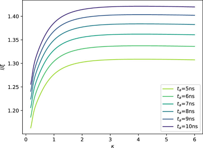
The phase-scrambling length l(87) (divided by ξ) as a function of the scaling parameter κ. A broad maximum is located near κ = 4.
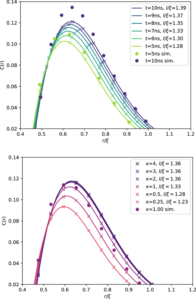
Top: the correlation for different annealing times ta at the scaling parameter κ = 1. Bottom: the correlation for different scaling parameters κ at ta = 7 ns. Theory has small deviations from the simulated (sim.) dynamics, consistent with corrections of O(1/ξ).
Special care is needed in the limit of small λ (κ), where the problem-energy scale diverges—particularly given that we consider dynamics initiated in a ground state at non-zero HP. For practical purposes, we might avoid these technicalities by considering extrapolation only to ‘small enough’ λ such that the statistical error is no longer dominated by ‘correctable’ noise (but by sampling error, systematic control errors, etc).
Experimental details
Several methods are presented in this section, alongside code examples sufficient for the reproduction of the main-text experiments in problem-Hamiltonian rescaling, and additional experimental data.
For simulation and the evaluation of λ(κ), we use the schedules shown in Fig. 6. These are developed based upon single and coupled-pair qubit experimental measurements, a parametric rfSQUID model, and a parametric (persistent-current based) mapping from an rfSQUID to Ising model (online documentation is available at https://docs.dwavesys.com/docs/latest/index.html. This includes QPU-specific properties (schedules and parameters)). This methodology leaves room for uncertainty and systematic errors18,19 (online documentation is available at https://docs.dwavesys.com/docs/latest/index.html. This includes QPU-specific properties (schedules and parameters)) that might explain some deviation in critical and post-critical phenomena of experimental results.
The schedules of the experimental and GA QPUs used in experiments parameterized by Γ(s) and ({mathcal{J}}(s)). The system Hamiltonian is (H(s)/h=-frac{1.8}{kappa }{mathcal{J}}(s){sum }_{i=0}^{L-1}{sigma }_{i}^{z}{sigma }_{i+1 ,(mod ,L)}^{z}-Gamma (s){sum }_{i=0}^{L-1}{sigma }_{i}^{x}), and h is the Planck constant and σx,y are the Pauli matrices and L is the system size L = 232 (experimental), 1024 (general access).
Zero-noise extrapolation was performed using linear extrapolation in T (Fig. 1), quadratic extrapolation in λ (Figs. 2 and 7), and linear extrapolation in λ (Figs. 3, 8, 9) to zero; in each case, we used least-square methods.
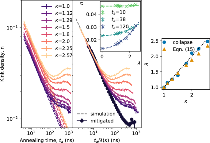
Error mitigation of kink density on the experimental Advantage2 system. (left) Kink density is measured for various annealing times ta and coupling energies J = −1.8/κ. An empirical rescaling of time is performed by collapsing fits of (rho propto {t}_{a}^{-1/2}) for ta < 10. (center) The collapse achieved by rescaling, circles represent the extrapolated points at fixed ta/λ. Center(Inset) ZNE is performed in λ, using a quadratic fit, Eq. (17). (right) λ(κ) obtained from collapse (circles) compared to those obtained from Eq. (15) (triangles).
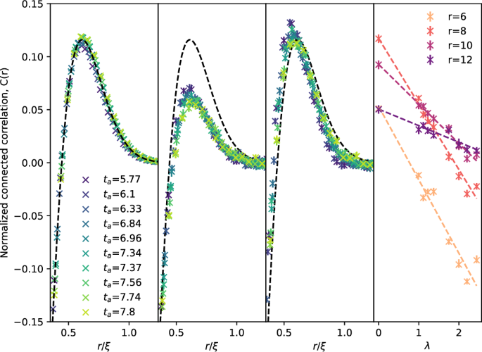
Mitigation of kink correlation on the experimental Advantage2 system. (Left) Simulation results are obtained for ({mathcal{C}}(r)); see “Methods—Simulation of dynamics” for details. Dashed line indicates a degree-10 polynomial that is replicated on the other panels to the right to facilitate comparison between theory and experiment. (Center-left) Unmitigated QA data (κ = 1) show correct qualitative behavior, but with a significantly flattened peak. (Center-right) Results obtained via linear ZNE to λ = 0 show good agreement with simulation, extrapolated curves are shifted to smaller r as is also observed for the GA Advantage2 prototype. (Right) We show example extrapolations for varying lattice distances r, with ta = 7.34 ns.
See description for Fig. 3. The kink density (top) is weakly dependent on the calibration refinement; there is small suppression in the kink density. The kink-correlation with calibration refinement at ta/λ(κ) = 8 ns (center) has enhanced peak-height, consistent with reduced disorder. We can combine calibration refinement with the collapse method for ta/λ(κ) = 8 ns, whereby λ kink-density is matched for all κ shown (described “Methods—Experimental details—Experimental Advantage2 prototype methodology at a scale L = 232”). This further enhances the peak height, but agreement with the 1-parameter theory (best fit l/ξ shown) is less convincing (at this ta); one can also observe that the data is clustered rather than linearly spaced in κ, indicating the perturbative (linear) approach is inappropriate.
Data and simulation curves shown in Fig. 3 are interpolated with a fitted four-parameter functional form, allowing reasonable agreement,
qualitatively matching the theory of “Methods—Critical and post-critical dynamics of the transverse field Ising chain”. Theory predicts, up to corrections O(1/ξ), parameters f = 9.31ξ/l3, 3π/l2, 1, 2π/ξ2.
Experimental Advantage2 prototype methodology at a scale L = 232
Quantum annealing experiments (Figs. 1, 7, and 8) were performed using a prototype D-Wave Advantage2 processor, with 232 flux qubits coupled in a one-dimensional periodic chain. Refinements of calibration are performed as previously detailed in the supplementary materials of ref. 18, and qualitatively matched to the description of the section “Experimental details—Calibration refinement method”47.
Average kink densities are measured over 20 programmings; 100 samples are taken in each programming. Kink correlations require more robust statistics, and are measured over 1000 programmings; 1000 samples are taken in each programming. All error bars represent 95% confidence intervals generated from bootstrap resampling of the 20 or 1000 programmings.
Qubit temperatures reported in Fig. 1 are measured by the population slope for uncoupled qubits subjected to a varying longitudinal field.
In the remainder of this section, we apply a problem-Hamiltonian rescaling on the same experimental Advantage2 system for which temperature extrapolation was performed (section “Zero-temperature extrapolation”), with a method assuming no knowledge of the schedule. This is an alternative to the schedule-derived method (15), and most appropriate when the schedule is not known with high confidence.
Figure 7. (left) shows measurements of kink density for different values of J = −1.8/κ as a function of annealing time. As expected, reducing the energy scale increases the number of kinks. Moreover, it increases the relative influence of the thermal environment as evidenced by the increasingly obvious deviation from (npropto {t}_{a}^{-1/2}) at high ta. Nonetheless, it is possible to rescale the horizontal axis ta → ta/λ, using λ as a free parameter, to collapse all of the data within some part of the diagram (the coherent annealing regime at small ta, specifically we choose ta < 10). We assume that this kink-density statistic is error-free, thereby eliminating the possibility of correction by extrapolation, but we obtain λ(κ) that can be applied at larger ta for kink density (or at any ta for other statistics such as C(r)). The resulting collapse is shown in Fig. 7(center) and the values of λ(κ) obtained by this collapse are plotted in Fig. 7(right) together with theoretical predictions using (15). Note that the collapse method will fail if static errors, such as Hamiltonian misspecification, significantly impact the coherent regime. The agreement between the empirical collapse and the annealing-schedule-inferred theoretical values of λ(κ) in the inset suggests that kink-density is insensitive to such errors, and conversely demonstrates that the schedule is relatively accurate with respect to the evaluation of (15) at experimental κ.
Given λ(κ) we can consider behavior outside of the collapsed regime, at large ta. Since the dominant noise is thermal, one should extrapolate using quadratic fits per Eq. (17). The inset in Fig. 7b illustrates this extrapolation for three different values of ta/λ. The black circles in the main panel show the result of this extrapolation. As in Fig. 1, the extrapolated points agree with the exact (npropto {t}_{a}^{-1/2}) behavior of larger ta. Thus one can successfully infer noise-free expectation values over a much broader range of annealing time than the ostensible coherent annealing regime.
We can also consider the kink correlation (18). For purposes of this section, we assume the kink-correlation with r normalized to ξ is weakly dependent on ta (as shown in Figs. 3 and 5) through the narrow range of ta studied, and we extrapolate to a curve averaged on ta. Figure 8 shows ({mathcal{C}}(r)) as a function of r normalized to the correlation length ξ = 1/n. Figure 8(left) illustrates the result obtained from simulation (BdG and DMRG are in agreement, as described in section “Simulation of dynamics”). Data is fitted with a 10th-order polynomial over the plot-range. Figure 8(center-right) illustrates the ZNE result, showing a significant improvement in alignment with the exact theoretical predictions (depicted by the solid lines), compared to unmitigated results (κ = 1, Fig. 8(center-left)). ({mathcal{C}}(r)) calculated by extrapolation, depicted in Fig. 8(center-right) exhibits a similar systematic deviation to that shown in Fig. 3, perhaps consistent with a reduced phase-scrambling-length scale (reduced post-critical dynamics). In Fig. 8(right), a few examples of extrapolation at different values of r are displayed, and unlike the case of thermal noise (Fig. 7), linear extrapolation works well, consistent with the correction of non-thermal noise sources.
GA Advantage2 prototype methodology at a scale L = 1024
In this section, we present details of the experimental method applied to the GA Advantage2_prototype2.3 QPU with supporting data. Code implementations are presented based on open-source repositories, principally the python package dwave-ocean-sdk (code examples rely upon dwave-ocean-sdk, an open-source Python repository hosted at https://github.com/dwavesystems/dwave-ocean-sdk)48,49. A connection to a QPU in the Leap quantum cloud service is established by  DWaveSampler() and can be configured to call any GA QPU: the QPU used in these experiments is an Advantage2 prototype. The 1024 spin-variables i must be mapped to QPU-specific qubits for programming purposes via an embedding. We require a set of qubits programmable as a ring, which amounts to solving a subgraph isomorphism problem49. This can be done with open-source tools typically in less than a second as follows
  Models with L > 1024 can be embedded, as above using additional time, or exploiting graph-specific insights. Embedding of smaller graphs is quicker, and can allow for parallelization. The ability to sample embeddings is useful to mitigate any locality-dependent errors. This can be achieved by creating the source and/or target graphs with shuffled variable and/or edge ordering before calling the deterministic subgraph search. Standard errors presented are determined with respect to variance between estimators on different programmings.
Given an anneal duration target ta (in microseconds, for κ = 1), and a rescaling κ, we can program and sample the QPU as  lam(κ) is the function (15), calculated from the published schedule.
For the kink-density experiments, we drew samples for five embeddings, a total of 5 programming, and 5000 samples. For the kink-correlation experiments we drew 16,000 samples for the same 5 embeddings, a total of 80 programmings and 80,000 samples. The kink density (inverse correlation length) fluctuates slightly as a function of κ, and the zero-noise extrapolated value differs from the simulation result. This can be accounted for by small errors in the schedule; the empirical method of the the section “Experimental details—Experimental Advantage2 prototype methodology at a scale L = 232” by which curves are collapsed can mitigate for such misspecification in principle. In Fig. 3, we calculate C(r) for fixed (programmed) ta at each κ, using the empirical kink correlations, and kink density (which is non-constant in κ).
Calibration refinement method
A refinement of the calibration, dependent on programmed Hamiltonian, is possible through exploiting symmetries. Coded examples of the method have been published47. Specifically, the transverse field Ising model is translationally invariant, and parity (defined by the operator ({prod }_{i}{sigma }_{i}^{x})) is a conserved quantity. As a consequence ({C}_{i}=langle {sigma }_{i}^{z}{sigma }_{i+1}^{z}rangle =bar{C}=1-2n), and ({m}_{i}=langle {sigma }_{i}^{z}rangle =0), respectively for all i in the noiseless limit. Deviations are a calibration failure that can be corrected by adjustment of the programmed J and flux bias (ϕ) to minimize sum square residuals: ({mathcal{O}}(phi )={sum }_{i}{m}_{i}^{2}) and ({mathcal{O}}(J)={sum }_{i}{({C}_{i}-bar{C})}^{2}). Stochastic local search is sufficient, given that the residuals are smooth functions of the calibration parameters about the correct calibration:
Here, {m, C, n} are sampling-based estimates on the tth programming, and α(t) is a learning rate.
For the presented data, we specify the learning rate as follows. In the first T/2 iterations, the learning rate is heuristically adapted so that the objective approaches a static value controlled by sampling error. On iterations for which ({{mathcal{O}}}_{phi }) (({{mathcal{O}}}_{J})) grows, the learning rate is decreased by a factor 1.1; otherwise it grows by the same factor. A fixed value of αJ ≲ 1, or αϕ ~ 10μΦ0, can also work well, but adaptation is useful for efficiency and stability, particularly at higher susceptibility parameterizations (lower kink rate). In the second T/2 iterations the learning rate decays polynomially as ~ 1/t, so that we mitigate for sampling noise, and obtain theoretical guarantees on convergence (up to non-static, but low-frequency variation beyond the experimental time scale, which is practically small).
The calibration is found to be converged for our purposes at T = 64. Given the refined calibration, we collect data per section “Experimental details—GA Advantage2 prototype methodology at a scale L = 1024”. In Fig. 9 we show the impacts on kink density and kink correlation. The impacts on the kink density are small: a modest decrease in the kink density is observed. The kink-correlation peak value is enhanced: this is consistent with reduced dephasing or control errors18,43. Whilst the result is improved, the calibration refinement does not substantially change the conclusions relative to experiments performed with the baseline calibration.
Similarly, we can use the method of the section “Experimental details—Experimental Advantage2 prototype methodology at a scale L = 232” to collapse data with matched ξ = 1/n. We can take the collected data, and interpolate C(r) so that kink density is matched at ta = 7ns, and extrapolate this collapsed data, as shown in Fig. 9. We combine this method with the calibration refinement, as was used on the experimental Advantage2 system. The result is a further enhancement of the peak C(r) height, which is compatible with reduced noise. However, the agreement with a coarsening theory based only on l/ξ is not improved (see departure from the fit curve). The data clearly shows signs of clustering in κ, indicating the linear (perturbative) fitting method has failed. Failure of the linear extrapolation ZNE method to match the coarsening theory at small ta seems to occur in conjunction with C(r) data clustering (as a function of κ), the origin of which requires further study.
Simulation of dynamics
Simulation results are obtained both by integration of the Bugolioubov-de Gennes equations (73), and matrix product state (MPS) dynamics. There is agreement between these methods. Results of simulation through the experimental range are shown in Fig. 10, and in other experiments for the GA Advantage2 system used in experiments. Results are well described by the analysis of IV C. In the experimental range the kink density is described by Kibble-Zurek theory; the kink correlation can be understood after accounting for post-critical dynamics with an additional length scale.
Simulation results for the kink correlation are shown for the GA Advantage2 system through relevant experimental parameters as a function of annealing time (top) and problem Hamiltonian rescaling (bottom). The peak value and position of the kink correlation curve grow larger with ta, and to a lesser extent with κ. The curves are well characterized by a kink density (determined by the Kibble-Zurek theory), and a phase-scrambling-length scale l, as described in section “Critical and post-critical dynamics of the transverse field Ising chain”; best fit values for l are shown. A two-length scale model predicts slightly smaller peak values than the simulation, but this discrepancy is consistent with corrections of order O(1/ξ, 1/L), and corrections vanish at larger scales as expected.
MPS dynamics are here simulated by the time-dependent variational principle (TDVP) with a two-site update50,51 using ITensor library52. We also compared the results against the WII method introduced in ref. 53 using the TenPy library54 and the local Krylov method55 (for details about this method in MPS language see ref. 56) implemented by the DMRG++ library57. Overall, we found that TDVP emerges as the most efficient method, providing converged results using the largest time step (dt=0.01 ns). For the lattice geometry, we adopted the same mapping from periodic to open chain used in ref. 18 as shown in Fig. 11a. We found a much better performance of the numerical simulations when using a local Hilbert space of two qubits (see Fig. 11b) for the MPS wave-functions.
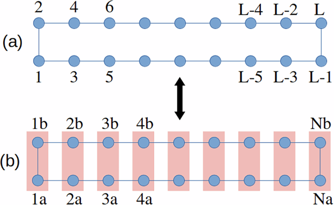
a Site ordering for MPS simulations of a periodic chain with one-qubit local Hilbert space. b Site ordering with a two-qubit local Hilbert space.
For the results shown in the main part of the manuscript, TDVP simulations were performed with a bond dimension D = 32 and a time step of 0.01 ns, with a maximum truncation error of 10−10.
Results can also be obtained, without the complications of a bond-dimension parameter, by a simple first- or second-order (Euler or Runge-Kutta) integration of the Bugoliobov de-Gennes equations at step size dt ~ 0.01 ns, as described in the section “Critical and post-critical dynamics of the transverse field Ising chain”. A DMRG method is also implemented validating the implementation. A strength of DMRG is the ability to efficiently generalize for inclusion of fields (hi), beyond first-neighbor couplings, or even explicit modeling of a bath, as analyzed in early works18.


Responses