Quantum locking of intrinsic spin squeezed state in Earth-field-range magnetometry

Sensitive measurements of magnetic fields in the Earth-field range is crucial to various real-world applications, including geological survey^1,2,3,4,5, biomedicine^6,7,8,9,10, fundamental physics experiments^{11,12,13,14,15}, and magnetic navigation^16,17,18,19. Alkali-metal atomic magnetometers are the outstanding candidates for such missions because of their high sensitivity, reaching the fT/(sqrt{{rm{Hz}}})^{20,21,22,23,24,25}. However, in the Earth-field range (50 μT), the nonlinear Zeeman (NLZ) effect produces splittings and asymmetries of magnetic-resonance lines, leading to the signal reduction and heading errors, and brings a well-known bottleneck limiting the sensitivity and accuracy of atomic magnetometry^{26,27,28,29,30,31,32,33}.

In order to tackle this bottleneck, the intuitive thinking is to eliminate the NLZ effect, while maintaining the spin coherence. Such an operation renders an Earth-field-range magnetometer with a sensitivity at the standard quantum limit (SQL)^{26,27,28,29,30,31,32,33}. Revisiting the spin dynamics in the Earth-field-range magnetometry with the NLZ effect, so far one has ignored an important fact that the intrinsic SSS exists due to the coupling of the electron spin and nuclear spin. However, as the atomic spin state sustains the continuous oscillation with the NLZ effect, the generated SSS exhibits the oscillating features on both the squeezing degree and squeezing axis, which prevent its direct observation and as well, accessibility to magnetic sensing.

How to lock and utilize such an oscillating SSS becomes essential to turn the drawback into the advantage, opening a new access to the development of Earth-field-range quantum sensing. To lock the SSS to the axis of the measurement quantity with optimal squeezing degree, here we develop the quantum locking technique which incorporates a dynamic decoupling (DD) sequence optimized by machine learning. The main used differential evolution (DE) algorithm is a global optimization algorithm that was inspired by a natural selection strategy³⁴ and can easily be applied in numerical simulations or quantum experiments^35,36,37. This model-free quantum locking technique has potential to be applied in other quantum technologies tackling decoherence such as performing error correction in quantum computation or maintaining the quantum state in quantum information. This intelligent Earth-field-range magnetometer, which automatically utilizes intrinsic SSS to achieve measurement sensitivity beyond the SQL, will inspires new ideas to those studying quantum metrology, Earth-field-range sensing, and quantum control, etc.

Spin squeezing with the NLZ effect

The NLZ effect originates from the hyperfine interaction (hat{i}cdot hat{j}) and the interaction between atom and magnetic field, where (hat{i}) is the nuclear spin, (hat{j}) is the electron spin. The eigenvalues of atomic Zeeman sublevels in a magnetic field B with electron quantum number J = 1/2 are given by the Breit-Rabi formula^38,39,

where ξ = (g_J + g_I)μ_BB/Δ, Δ is the hyperfine-structure energy splitting, I is the quantum number of nuclear spin, g_J and g_I are the electron and nuclear Landég factors, respectively, μ_B is the Bohr magneton, B is the magnetic field intensity, and the ±refers to the f = I ± J hyperfine components for a single atom. In Earth’s magnetic field, the nonlinear term in Eq. (1) cannot be neglectable, so we expand the eigenvalues to the second order of magnetic field B. For state ⁸⁷Rb5²S_1/2f = 2, the energy level keeping only the magnetic field dependence is:

Since the linear Zeeman effect shows linear dependence with magnetic quantum number m and the NLZ effect shows quadratic dependence with m, the Hamiltonian of atom-magnetic field interaction with the leading magnetic field B along the (hat{tilde{z}}) axis can be described as:

where ℏ is Plank’s constant, ({hat{f}}_{z}) is the angular momentum along (hat{z}) axis of a single atom, Ω_L = γ B = (μ_BB)/(2ℏ) is the Larmor frequency, (omega ={({mu }_{B}B)}^{2}/(4{hslash }^{2}Delta )) is the quantum-beat revival frequency, γ is the gyromagnetic ratio. The first term in Eq. (3) denotes the Larmor precession. The second term in Eq. (3) has the same form as the one-axis spin twisting introduced by Kitagaa and Ueda⁴⁰. Note that the SSS induced by the NLZ effect coming from the total angular momentum (hat{f}) of a single atom^41,42,43, whereas Kitagawa and Ueda refers to the collective angular momentum (hat{F}) of an ensemble of atoms.

In the rotating frame, considering a coherent spin state (CSS) stretched along the (hat{tilde{y}}) axis for f = 2 system evolves under the free evolution Hamiltonian ({hat{widetilde{H}}}_{B}=-hslash omega {hat{tilde{f}}}_{z}^{2}), where the operator (hat{tilde{o}}) denotes the operator (hat{o}) in the rotating frame (Specific formulas are demonstrated in the Supplementary Note 2). For a spin state polarized perpendicular to the magnetic field, ({hat{widetilde{H}}}_{B}) induces coupling between the eigenstates of the angular momentum along the direction of the polarized spin and causes squeezing of the spin state. The squeezing angle ν, defined as the angle between the optimal squeezing axis and (hat{tilde{x}}) axis, is calculated by (nu =pi /2-1/2arctan (Y/X)), where (X=1-{cos }^{2f-2}(2omega t)), (Y=4sin (omega t){cos }^{2f-2}(omega t)). The optimal squeezing axis of the SSS varies at different times. The green line in Fig. 1a shows the minimum noise along the optimal squeezing axis at different times, illustrating that the squeezing degree changes over time as well.

a The noise of the spin projections along the optimal squeezing axis (green line) and the noise of ({hat{widetilde{F}}}_{x}) (red line) at different times. The dashed line is the noise of CSS f/2 for single atom. As the spin squeezing arises from the single-atom effect, the atom number N is set to 1 in the simulation. b The metrological gain along the optimal squeezing axis at different times. The red star denotes optimal squeezing point to be locked.

Full size image

In an atomic magnetometer, the measurement quantity is the Larmor precession frequency, which is typically measured through finding the time between two zero crossings of a collective of oscillating spin component²². For an atomic ensemble with N atoms, the collective angular momentum components are ({hat{widetilde{F}}}_{x}=mathop{sum }nolimits_{r = 1}^{N}{hat{tilde{f}}}_{x}^{(r)}) and ({hat{widetilde{F}}}_{y}=mathop{sum }nolimits_{r = 1}^{N}{hat{tilde{f}}}_{y}^{(r)}). While no atom-atom entanglement presents, the signal and noise of the corresponding magnetic measurement are scaled as (| partial langle {hat{widetilde{F}}}_{x}rangle /partial {theta }_{L}| =langle {hat{widetilde{F}}}_{y}rangle =Nlangle {hat{tilde{f}}}_{y}rangle) and (Delta {hat{widetilde{F}}}_{x}=sqrt{{rm{Var}}({hat{widetilde{F}}}_{x})}=sqrt{N{rm{Var}}({hat{tilde{f}}}_{x})}), respectively, where θ_L = Ω_LT₂ = γBT₂ is the phase of Larmor precession, T₂ is the coherence time of atomic spin. The sensitivity of the atomic magnetometry is

where (zeta =sqrt{{rm{Var}}({hat{tilde{f}}}_{x})}/langle {hat{tilde{f}}}_{y}rangle) is the spin-squeezing parameter of single atom. With CSS injection, Eq. (4) determines the SQL for atomic magnetometry (Delta {B}_{{rm{SQL}}}=1/(gamma {T}_{2}sqrt{2Nf}))^{20,41,43,44,45,46,47} (see details in Supplementary Note 1). In this paper, we focus on the quantum enhancement of ζ which arises from nuclear-electronic spin entanglement^41,42,43 (see details in Supplementary Note 3).

To employ the SSS in quantum metrology, it is essential to match the angular momentum component with minimum noise to the measurement quantity. The red line in Fig. 1a shows the noise ({rm{Var}}({hat{widetilde{F}}}_{x})) of the measurement quantity ({hat{widetilde{F}}}_{x}) with NLZ effect, which always exceeds the fluctuation of CSS. That is because the optimal squeezing axis of this type of SSS is not along the observable ({hat{widetilde{F}}}_{x}). We can rotate the SSS along the –(hat{tilde{y}}) axis by ν to align the optimal squeezing axis with the axis of ({hat{widetilde{F}}}_{x}), thereby ensuring that ({hat{widetilde{F}}}_{x}) has the minimum noise. The quantum enhancement of magnetic field measurement arises from squeezing of the noise.

After the rotation operation with angle ν, we calculate the resulting single-shot sensitivity of the magnetic field measurement with N atoms⁴⁸

see details in Supplementary Note 2. In order to intuitively represent the advantage of the SSS injection, we use the metrological gain defined as (g={(Delta {B}_{{rm{SQL}}}/Delta {B}_{{rm{SSS}}})}^{2})⁴⁹ to represent the quantum enhancement for the sensitivity. The metrological gain is then (g={(cos omega t)}^{2(2f-1)}/[1+(1/2)(f-1/2)(X-sqrt{{X}^{2}+{Y}^{2}})]). Since the spin squeezing arises from the single-atom effect, the metrological gain is independent of N. For f = 2 system, the metrological gain is shown in Fig. 1b. The maximum metrological gain defined as the optimal squeezing point approaches 2.9 dB at ωt = 0.34. Note that the maximum gain [Fig. 1b] doesn’t occur at the minimum noise [Fig. 1a], because the signal and the noise have different time dependencies.

The maximum metrological gain g_m with respect to ωt is scalable with the quantum number of total angular momentum f for a single atom. Figure 2 plots g_m as a function of f. Relatively large values of f available are f = 4 in the ground state of Cs and f = 12.5 in a metastable state of Dy⁵⁰, corresponding to a maximum metrological gain by 4.5 dB and 7.7 dB, respectively, which are comparable to the reported ones with multi-atom collective spin squeezing^44,51. The maximum metrological gain can scale up even higher with larger f such as in Rydberg atoms and in molecules⁴¹.

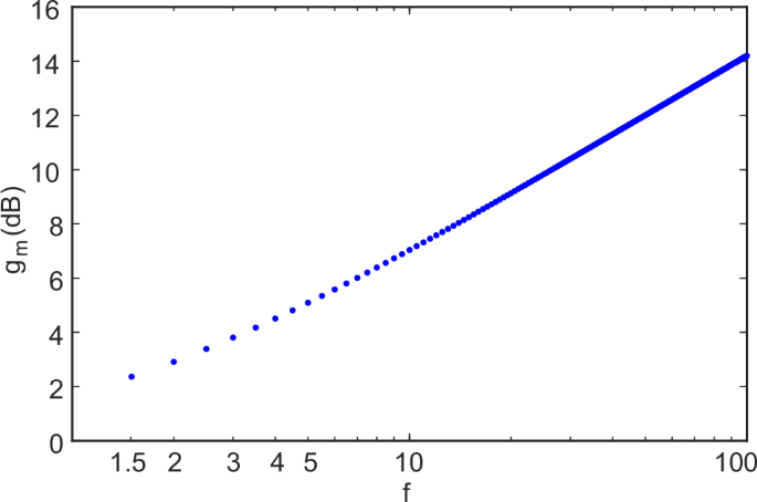
The maximum metrological gain g_m varies with f.

Full size image

Quantum spin locking

The SSS produced by the NLZ effect could help improve the sensitivity of atomic magnetometry. However, because the NLZ effect always exists, the SSS keeps evolving. To lock the SSS at the optimal squeezing point [the star in Fig. 1b], we develop the quantum locking method, which is a machine-learning-assisted DD technique.

We set the wavefunction of the SSS to be locked as (leftvert Psi (0)rightrangle). Figure 3 shows the principle of the quantum spin locking scheme in the form of the real-time fidelity ({{mathcal{F}}}_{r}={rm{Tr}}| sqrt{sqrt{{rho }_{0}}{rho }_{t}sqrt{{rho }_{0}}}{| }^{2}) between the SSS and the state at time t. ({rho }_{0}=leftvert Psi (0)rightrangle leftlangle Psi (0)rightvert) is the density matrix of the SSS. ρ_t is the density matrix of spin state at time t. If the SSS evolves freely with the NLZ effect, the SSS collapses and revives periodically, as the blue line in Fig. 3 shown. While, in the quantum locking scheme, utilizing the periodic property of spin evolution under the NLZ effect, the SSS can be locked by taking the shortcut from Ψ(t₁) to Ψ(2π − t₁), which can be achieved by the spin evolution with the DD sequence ({hat{widetilde{U}}}_{DD}(T)) (as the red line in Fig. 3 shown), where T is the period of one DD cycle. More detail is discussed in Supplementary Note 8.

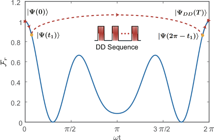
The red star at the starting point is the SSS (leftvert Psi (0)rightrangle) to be locked. The blue line represents the real-time fidelity of the SSS oscillating at the period 2π with the NLZ effect. The red line is the path of the state evolution in the DD process. The SSS firstly evolves to (leftvert Psi ({t}_{1})rightrangle), then slips to (leftvert Psi (2pi -{t}_{1})rightrangle) and finally revivals to the state (leftvert {Psi }_{DD}(T)rightrangle). T is the period of the DD sequence and is set substantially shorter than the revival period 2π/ω. Ω_L = 2π, Ω_L/ω = 20000, TΩ_L = 2π × 2000.

Full size image

The DD sequence consists p instaneous rotation pulses ({hat{Pi }}^{d}({chi }_{i}),(i=1ldots p)) following the free evolution ({hat{widetilde{U}}}_{F}(T/p)), where ({hat{Pi }}^{d}({chi }_{i})={e}^{-i{chi }_{i}{hat{tilde{f}}}_{d}}) is the pulsed rotation evolution operator, ({hat{widetilde{U}}}_{F}(T/p)={e}^{-i{hat{widetilde{H}}}_{B}T/phslash }) is the free evolution operator. The pulse is applied by a radio-frequency (RF) magnetic field in the laboratory frame (a static magnetic field in the rotating frame). (d=pm hat{tilde{x}},pm hat{tilde{y}},pm hat{tilde{z}}) is the rotation direction in the rotating frame which is decided by the phase of RF field, χ_i is the rotation angle of the i-th pulse. To ensure that the atomic spin remains stretched along the (hat{tilde{y}}) direction and that as many atomic spins as possible can be used to sense the magnetic field, the pulses in the DD sequence are all along the –(hat{tilde{y}}) axis. Hence, the DD sequence takes the form

For a specific angular momentum f, the DD performance is a function of parameters T, p, and χ_i (i = 1…p). In the experiment, there are some restrictive conditions for the values of these parameters. The DD period T should be substantially shorter than the revival period 2π/ω to ensure that the SSS experiences enough DD cycles and keeps squeezed most of the time. Theoretically, the rotation angle χ_i is arbitrary. Considering the running speed of the algorithm and the convenience of pulse design in the experiment, χ_i is set to be nπ/36 (step length is 5 degrees), where n is an integer. The relationship between the rotation angle χ_i and the pulse length t_i, is formulated as ({chi }_{i}=mathop{int}nolimits_{0}^{{t}_{i}}{Omega }_{i}(t)dt), where Ω_i(t) denotes the energy distribution of the ith pulse. The pulse length t_i should be considerably shorter than the free evolution time T/p to satisfy the instaneous rotation condition and substantially longer than the Larmor period to satisfy the rotation wave approximation condition⁵². Considering the Larmor frequency, the quantum-beat revival frequency of ⁸⁷Rb in the Earth-field range and the restrictive conditions mentioned above, we choose Ω_L/ω = 20000, TΩ_L = 2π × 2000, and p = 10 for the DD sequence optimization.

We introduce the final state ({{mathcal{F}}}_{f}={rm{Tr}}| sqrt{sqrt{{rho }_{0}}{rho }_{T}sqrt{{rho }_{0}}}{| }^{2}) to evaluate the DD performance^53,54,55, where ({rho }_{T}={hat{widetilde{U}}}_{DD}(T)leftvert Psi (0)rightrangle leftlangle Psi (0)rightvert {hat{widetilde{U}}}_{DD}^{dagger }(T)) is the density matrix of spin state after one DD sequence. For the locking of the SSS, our goal is to determine the optimal χ_i in the DD sequence so that the fidelity ({{mathcal{F}}}_{f}) is as close to 1 as possible. The DE algorithm is used to obtain the DD sequence. The target function is the infidelity (1-{{mathcal{F}}}_{f}). The spin state is measured by the Faraday interaction between the probe light and the atomic system (see “Methods” for details). The fidelity can be obtained by the state tomography through varying the propagation direction of the probe light^56,57,58. Our pulse sequence design task can be seen as a kind of multi-parameter optimization with discrete variables. As a gradient-free algorithm, the DE algorithm is a powerful choice, which is not easily trapped in a local optimum solution³⁴. The framework of the proposed approach is shown in Fig. 4. For given T and p, we generate an initial population containing a series of DD sequences with random rotation angles. The DD sequences are applied to the atomic system by the coils in the form of the RF field pulses. The main operations are mutation, crossover, and selection. In the mutation operation, three DD sequences are randomly selected from the population as the mutation sources and combined to reproduce the mutation sequence [see Eq. (12) in “Methods”]. The rotation angles in the original DD sequence are partially replaced by the ones in the mutation sequence to derive the test sequence [see Eq. (13) in “Methods”], which is the crossover operation. In the selection process, the target function values of the test sequence and the original sequence are compared, and the sequence with the better value is retained to the next optimization loop. The three operations mentioned above are performed once on each DD sequence in every loop to update the population. After a number of iterations, the algorithm gradually converges to the optimal sequence

in which T is set as 1/10 revival periods.

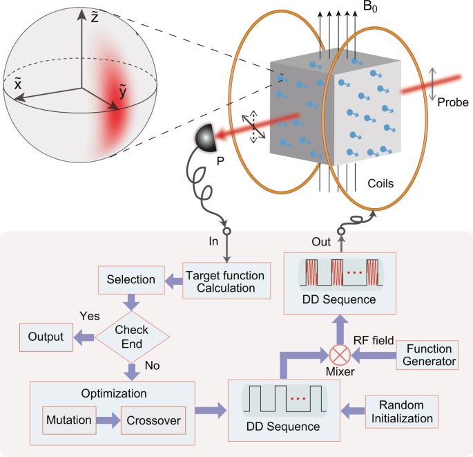
With the leading magnetic field B₀ along the (hat{tilde{z}}) axis, the atomic spins oscillate in the (hat{x}-hat{y}) plane at Larmor frequency in the laboratory frame and are orientated along the (hat{tilde{y}}) axis in the rotating frame. With the NLZ effect, the spins are squeezed along the optimal squeezing axis. After the rotation operation with angle ν, the ({hat{widetilde{F}}}_{x}) is squeezed as represented on the Bloch sphere. A sequence of pulses optimized by the DE algorithm are applied in the form of the RF field pulses along the –(hat{tilde{y}}) axis to lock the SSS. P is the polarimeter used to measure the spin projection of the atomic state for the target function calculation. The end condition is when we reach the maximum generation. More detail is discussed in Methods.

Full size image

The dynamic evolution of the atomic state is illustrated by calculating the quasi-probability distribution⁴⁰. Figure 5a–c represent the generation of the SSS and (c–o) describe the evolution of the SSS during the DD sequence in Eq. (7). The fidelity between the states (c) and (o) is 99.99%, which proves the success of this DD sequence.

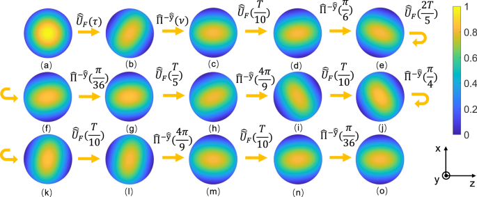
The quasi-probability distribution of the atomic spin state Q(θ, ϕ) = ∣〈θ, ϕ∣Ψ(t)〉∣², where (leftvert theta ,phi rightrangle) is the CSS, θ is the polar angle ranging from [0, π], ϕ is the azimuthal angle ranging from [0, 2π], and (leftvert Psi (t)rightrangle) is the atomic wavefunction at time t. a The initial CSS stretched along the (hat{tilde{y}}) axis. b The optimal SSS. c The SSS with the optimal squeezing axis along the (hat{tilde{x}}) axis after the rotation operation. d–o The evolution of the SSS (c) during one DD cycle. τ is the time when the most squeezed spin state occurs and ωτ = 0.34. T is the period of the DD sequence.

Full size image

Magnetic field measurement with the SSS

To measure the magnetic field, a linearly polarized probe light is utilized to measure the spin component projection along the (hat{x}) axis by the first order atom-light interaction (see “Methods” for details). After the probe light propagating through the atomic sensors, the polarization angle of the probe light is rotated. From the polarization rotation signal detected by a polarimeter, we therefore obtain the spin component ({hat{F}}_{x}) which oscillates at Larmor frequency of leading magnetic field, as shown in Fig. 4. Here, we measure the magnetic field perturbation δB in the leading magnetic field B₀. In the locking stage, the frequency of the RF field is the same as the Larmor frequency of B₀. In the measurement stage, without the RF field, the Larmor precession frequency can directly reflect δB.

There are two protocols to apply the probe light pulse. The SSS can be locked during an interval of darkness permitting the spin state to precess in the presence of the static magnetic field and DD pulses. A probe pulse is then applied for readout⁵⁹, as shown in the protocol I in the Fig. 6a. In this condition, the power broadening and back-action induced by the probe light is avoided by sacrificing the measurement time t_p1. While, in a conventional magnetometry, the probe light is applied in the whole time t_p2 and monitor the Larmor procession, as shown in the protocol II in the Fig. 6a. In this protocol, high fidelity during the whole measurement process is required and the optimal DD sequence is obtained by maximize the (overline{{{mathcal{F}}}_{r}}), where (overline{{{mathcal{F}}}_{r}}) is the average real-time fidelity during the DD operation.

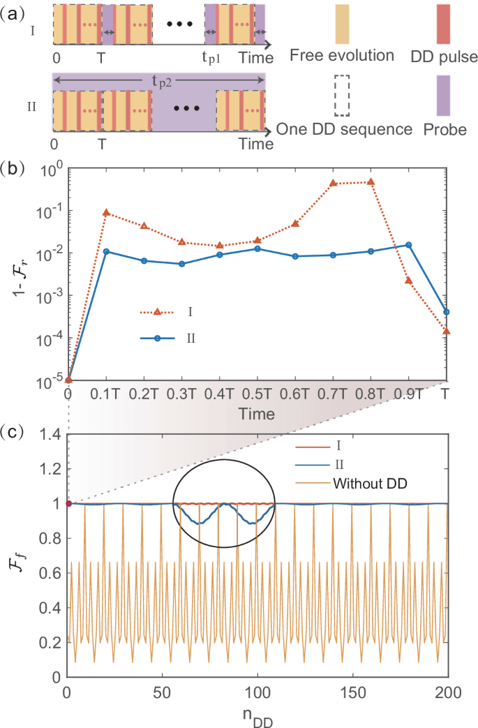
a The sequence in different measurement protocols. t_p1 and t_p2 are the total time of the probe light in different protocols. b The real-time infidelity (1-{{mathcal{F}}}_{r}) after each rotation operation in one DD sequence in different measurement protocols. T is set as 1/10 revival periods. c The final fidelity ({{mathcal{F}}}_{f}) during 200 DD cycles in different protocols. Inset is the zoom in picture. n_DD denotes the number of the DD cycles.

Full size image

Figure 6b compares the real-time infidelity (1-{{mathcal{F}}}_{r}) after each rotation operation in one DD sequence for the two measurement protocols. In protocol I, the (overline{{{mathcal{F}}}_{r}}) during the DD operation is low, but the spin state is well locked at the end of the DD sequence with a final fidelity of 99.99%. In protocol II, the fidelity of the final state 99.83% is lower than that in protocol I, while the (overline{{{mathcal{F}}}_{r}}) is better.

An effective DD sequence is also essential to ensure a high fidelity for a long-time duration, which guarantees sufficient time to perform the measurement. Without the DD sequence, the fidelity periodically oscillates due to the NLZ effect as shown in Fig. 6c; while with DD sequence, the fidelity remains in the range [99.97%, 99.99%] in protocol I and [99.28%, 99.99%] in protocol II. The long-time stability of the locked SSS in protocol I is better than that in protocol II, even during several hundred cycles. The quantum spin locking scheme is flexibly adapted to different measurement protocols as we choose appropriate target function depending on the requirements for the SSS in the measurement process.

In addition, a magnetic field gradient is inevitable in a natural environment. The phase perturbation due to an inhomogeneous magnetic field accumulates over time and causes a small spin-orientation broadening along the spin state. Dephasing due to an inhomogeneous magnetic field can be largely suppressed by using the Hahn echo^27,60, where a ({hat{Pi }}^{tilde{y}}(pi )) pulse is applied during the free-evolution interval. In quantum locking scheme, to remove the magnetic field gradient simultaneously, the ({hat{Pi }}^{tilde{y}}(pi )) pulse could be added in each free evolution ({hat{widetilde{U}}}_{F}(T/p)) of DD sequence. Notably, the ({hat{Pi }}^{tilde{y}}(pi )) pulses have no influence on the quantum locking scheme²⁷.

To conclude, in this paper, the intelligent Earth-field-range magnetometer, which automatically utilizes intrinsic SSS to achieve measurement sensitivity beyond the SQL is proposed. We turn the NLZ effect, which limits the sensitivity of the Earth-field-range magnetometer into a valuable technique for quantum enhancement of magnetic sensing. Due to the continuous collapse and revival of the atomic state induced by the NLZ effect, the SSS oscillates over time and is not typically used in experiments. This issue can be solved by locking the SSS with periodic pulsed modulations. The pulse sequence is calculated by the DE algorithm.

There are three steps to build such a quantum-enhanced magnetometer in the Earth-field range. First, the state evolves freely to generate the SSS; then, at the time of the optimal squeezing point, a rotation operation is performed to align the optimal squeezing axis with the measurement axis; and finally, a DD sequence is applied to lock the SSS and the magnetic measurement is implemented. With the help of the SSS injection, the noise of the magnetic resonance can be reduced; in addition, the application of the quantum locking technique cancels the extra NLZ effect, which increases the magnetic resonance’s amplitude and narrows its linewidth. Supposing the atoms in a 1 cm³ cell working in the room temperature, the atom number is 1.42 × 10^{10 61}. With the coherence time of 10 ms, the SQL is 5.99 fT/(sqrt{{rm{Hz}}}). For ⁸⁷Rb in the Earth’s magnetic field (50 μT), due to the NLZ effect, the spin state undergoes rapid collapse with an effective coherence time of 1.82 ms, which leads to a sensitivity of 14.04 fT/(sqrt{{rm{Hz}}}). By using the quantum locking technique, with the benefit of both maintaining the coherence time and spin squeezing, the sensitivity reaches 4.29 fT/(sqrt{{rm{Hz}}}). Such quantum-enhanced magnetometry is promising for practical applications in the Earth-field range.

The quantum locking technique proposed in this paper can, without loss of generality, be extended to lock the other spin system with quadratic interaction^62,63 or large-f SSS with high metrological gain. In this work, B₀ is fixed and δB is considered as a minor perturbation. In the case of substantial variation of the magnetic field, the frequency of the RF field applied each time needs to be adjusted based on the result of the previous measurement. The measured Larmor frequency serves as feedback to correct the RF field frequency with the Larmor frequency. Similar closed-loop schemes have been achieved in conventional optically pumped magnetometry by self-oscillating⁶⁴ or phase lock loop⁶⁵ which lock the frequency of driving field to the Larmor frequency. Then the uncertainty of the previous measurement would influence the overall measurement performance. In our system, the single-shot sensitivity is at the level of 1 pT. This level of uncertainty does not notably impede the metrological gain and DD operations. More detail is discussed in Methods. Here we study the SSS generated from a single atom. By generating entanglement between atoms, the metrological gain can be further improved⁵¹. The protocol proposed here works as a scalar magnetometer by measuring the Larmor frequency of atomic spins which is intrinsically sensitive to the magnitude of an applied field rather than its projection along a particular direction. There are several ways to derive information of magnetic field direction, converting a scalar magnetometer into a vector magnetometer^66,67. With the magnetic field much larger than Earth-field range, higher order nonlinear effect would arise. The spin dynamic in this condition needs to be further studied.

Optimization algorithm

In our work, a DD sequence is used to lock the SSS with high fidelity. The DE algorithm is used to determine the optimal rotation angles in the DD sequence. The target function (f(overrightarrow{x})=1-{{mathcal{F}}}_{f}) is served as the cost function of the DE algorithm, where ({{mathcal{F}}}_{f}) is the fidelity calculated after the DD sequence. The variable (overrightarrow{x}) denotes a DD sequence containing p rotation angles and is written in the form of a vector as

where xⁱ(i = 1, 2, …, p) is the i-th rotation angle in the sequence.

The domain of the function (f(overrightarrow{x})) with maximum rotation angle ({overrightarrow{x}}_{max}) and the minimum rotation angle ({overrightarrow{x}}_{min}) is defined as

Our target is to find the minimum of the target function (f(overrightarrow{x})) within the defined domain.

First, an initial population containing M DD sequences with p random rotation angles is generated. The j-th sequence in the k-th loop of the population can be expressed as

where Q is the maximum number of the loop. The j-th sequence in the first loop ({overrightarrow{x}}_{j,1}) is obtained randomly:

where rand(0, 1) is a uniform random number between 0 and 1.

The next operation is the mutation operation. Three DD sequences are randomly selected from the population as the mutation sources and combined to reproduce the mutation sequence. The mutation sequence ({overrightarrow{v}}_{j,k}) for the j-th sequence in the k-th loop is obtained by

where ({r}_{1}^{j}), ({r}_{2}^{j}) and ({r}_{3}^{j}) are randomly generated integers that are not equal to j, F_s is a preset scaling factor in the range 0 < F_s < 1.

Then, the crossover operation is applied. The rotation angles in the original DD sequence ({overrightarrow{x}}_{j,k}) are partially replaced by the ones in the mutation sequence ({overrightarrow{v}}_{j,k}) to derive the test sequence ({overrightarrow{u}}_{j,k}) as follows:

where i_rand is a random integer, ({r}_{j}^{i}) is a random number between 0 and 1, and P_cr is the predefined crossover probability.

Finally, in the selection process, the target function value (f({overrightarrow{u}}_{j,k})) is compared with (f({overrightarrow{x}}_{j,k})). The sequence with smaller value is retained in the next loop i.e.,

The three operations are performed once on each DD sequence in every loop to update the population. After a number of iterations, the algorithm gradually converges to the optimal sequence until the number of loop reaches a preset threshold.

In our case, the dimension p of (overrightarrow{x}) is set to 10 and the rotation angle is set to be nπ/36, where n is an integer. Considering the running speed of the algorithm, the domain of (overrightarrow{x}) is set to [0, π/2]. The size of the population M is set to 100. The maximum number of loop Q is set to 1000. The scaling factor F_s is set to 0.5. The crossover rate P_cr is set to 0.3.

Spin state measurement

To measure the atomic spin state and thus obtain the Larmor frequency of the atomic spin, a far-off resonant and linear-polarized light propagating along the (hat{x}) axis is introduced. The proprieties of the probe light can be described by the Stokes operators ({hat{S}}_{x}=1/2({hat{a}}_{x}^{dagger }{hat{a}}_{x}-{hat{a}}_{y}^{dagger }{hat{a}}_{y})), ({hat{S}}_{y}=({hat{a}}_{x}^{dagger }{hat{a}}_{y}+{hat{a}}_{y}^{dagger }{hat{a}}_{x})), ({hat{S}}_{z}=i/2({hat{a}}_{y}^{dagger }{hat{a}}_{x}-{hat{a}}_{x}^{dagger }{hat{a}}_{y})). The Hamiltonian of atom-light interaction (hat{{H}_{L}}) can be approximated to the first order:

where, κ is the first order coupling constant of the atom-light interaction. The input-output relation of ({hat{S}}_{y}) is:

With this interaction, the spin projection along the (hat{x}) axis can be measured by monitoring the ({hat{S}}_{y}^{out}) of the probe light. The other spin components can be measured by changing the propagation direction of the probe light. The fidelity can be derived by the state tomography.

We also notice that the atom-light interaction would induce back action to the atomic spins. The input-output relation of spin operators is:

Although the probe light is linearly polarized i.e., (langle {hat{S}}_{z}rangle =0), it will have quantum fluctuations in the degree of the circular polarization. With a macroscopic spin polarized along the (hat{z}) ((hat{y})) axis, the fluctuation of optical field is mapped to the spin fluctuation (hat{{F}_{y}}) ((hat{{F}_{z}})). Since the spin in our system is oscillating on the (hat{x}-hat{y}) plane, the back action is always acted on ({hat{F}}_{z}) which is the anti-squeezed component of the SSS mentioned in the last section. So the back action does not affect the squeezing of the spin state.

Closed-loop scheme with substantial variation of the magnetic field

In the magnetic field measurement, we measure the magnetic field perturbation δB in the leading magnetic field B₀. In the main text, B₀ is fixed and δB is considered as a minor perturbation. In this case, the frequency of the RF field is set to the same as the Larmor frequency of B₀ and the angle ν is also derived from B₀. While, in the case of substantial variation of the magnetic field, if the RF field frequency and angle ν are still derived from B₀, the initially generated SSS and the DD performance will be affected by the variation δB of the magnetic field. This issue can be addressed using closed-loop scheme. The measured Larmor frequency is used as feedback to adjust the frequency of RF field in order to lock it to the Larmor frequency, as shown in Fig. 7. Then the uncertainty of previous measurement would influence the measurement performance. In each measurement process, despite possible degradation caused by δB in the SSS generation and the DD performance, there exists a range of δB for maintaining the metrological gain. To guarantee quantum enhancement in each measurement, the single-shot measurement uncertainty should be smaller than the range of magnetic deviation maintaining metrological gain.

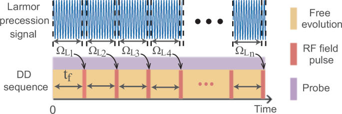
The blue line is the Larmor precession signal. The measurement process is implemented during the free evolution process lasting t_f. Ω_Ln(n = 1, 2, 3…) are the measured real-time Larmor frequency. The frequency of the RF field pulse is adjusted to the Larmor frequency of the previous measurement.

Full size image

The single-shot measurement uncertainty is calculated by (1/(sqrt{g}gamma {t}_{f}sqrt{2Nf})). Here, t_f = T/p is the free evolution time since the measurement process is implemented during the free evolution process as shown in Fig. 7. Based on the pulse length discussed in the Supplementary Note 5, t_f could be 400 μs. With atom number N = 1.42 × 10¹⁰, the single-shot measurement uncertainty is 1 pT.

To evaluate the impact brought by the measurement uncertainty, we calculate the metrological gain g obtained from the initial SSS and the SSS after 200 DD cycles change at different magnetic field deviation ratios δB/B₀ within the range of [−5 × 10⁻⁵, 5 × 10⁻⁵], corresponding to δB in [−2.5 nT, 2.5 nT], as B₀ = 50 μT (the Earth’s magnetic field). The metrological gain is (g={(Delta {B}_{{rm{SQL}}}/Delta {B}_{{rm{SSS}}})}^{2}={[langle {hat{widetilde{F}}}_{y}rangle /(sqrt{2Nf}Delta {hat{widetilde{F}}}_{x})]}^{2}). In the frame rotating at the RF field frequency ω_RF which is set as the Larmor frequency ω_RF = Ω_L = γ B₀, the Hamiltonian becomes ({hat{widetilde{H}}}_{B}=gamma delta B{hat{tilde{f}}}_{z}-hslash omega {hat{tilde{f}}}_{z}^{2}). We still utilize the formula of ν derived from B₀ and the DD sequence of Eq. (7) in the main text to generate and lock the SSS. The resulting metrological gains are shown in Fig. 8. The generation process of the SSS contains only one RF field pulse to rotate the squeezing axis to the direction of the measurement quantity, while the DD process contains 200 DD cycles each has 10 pulses. Therefore, the metrological gain achieved by the locked SSS after 200 DD cycles is more easily to be affected by the magnetic field deviation ratios, exhibiting an oscillating feature, as shown in the red line of Fig. 8. Even so, the metrological gain shows robustness in a wide range of δB in [−50 pT, 50 pT], as shown in the insert of Fig. 8. This range is much bigger than the single-shot measurement uncertainty of 1 pT.

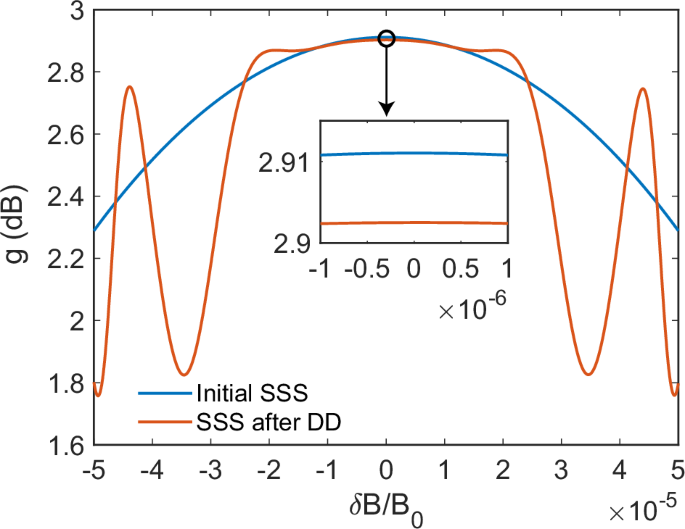
The metrological gain at different magnetic field deviation ratios δB/B₀. The blue line denotes the metrological gain achieved by the initially generated SSS. The red line denotes the metrological gain achieved by the locked SSS after 200 DD cycles. Insert shows the case of δB in the range of [−50 pT, 50 pT] with B₀ = 50 μT.

Full size image