Quantum Zeno Monte Carlo for computing observables

Introduction
The quantum computer1,2,3 utilizes quantum algorithms to tackle computationally challenging problems, offering potential solutions to classically hard problems. A significant challenge lies in finding Hamiltonian eigenstates and their physical properties4, crucial for material design and quantum machine learning implementation. By providing an initial state sufficiently close to the target eigenstate, this problem can be solved within polynomial quantum time5,6 with a fully fault-tolerant quantum computer (FTQC)7,8. However, the preceding decades have been marked by the noisy intermediate-scale quantum (NISQ) era9 rather than the FTQC era. Due to substantial device noise, quantum algorithms for NISQ systems prioritize noise resilience, leading to the dominance of ansatz-based algorithms10,11,12 without provable polynomial complexity.
The emergence of quantum devices with 48 logical qubits13 marks the start of error-corrected quantum computing. These devices, along with their future advancements, have the potential to showcase quantum advantage, bridging the gap between NISQ and FTQC eras. Early error-corrected quantum computers are expected to handle longer quantum circuits than NISQ devices and execute quantum algorithms with polynomial complexity. However, algorithms designed for the FTQC era may not be suitable for early error-corrected quantum computers, as they still face device noise due to limited error corrections. As a result, developing new quantum algorithms that cost polynomial quantum time and are resilient to noise shows promise for achieving quantum advantage in early error-corrected quantum computers.
We introduce the quantum Zeno Monte Carlo (QZMC) algorithm. This algorithm is robust against device noise as well as Trotter error. Furthermore, this algorithm enables the computation of static as well as dynamic physical properties for gapped quantum systems within polynomial quantum time. Notably, QZMC does not necessitate overlap between the initial state and the target state, nor does it require variational parameters. We validate its resilience to device noise by implementing it on IBM’s NISQ devices for systems with up to 12 qubits. We also demonstrate its resilience to the Trotter error and the polynomial dependence of its computational cost by numerical demonstration on a noiseless quantum computer simulator. Our method’s resilience to Trotter errors allows us to compute eigenstate properties with shallower circuits, as demonstrated in comparisons with recent phase estimation techniques14,15.
Results
The Quantum Zeno Monte Carlo algorithm draws inspiration from the quantum Zeno effect16. This is the phenomenon that repeated measurements slow down state transitions. We briefly outline this effect: A system varying with a continuous variable λ is represented by the state (vert {psi }_{lambda }rangle). Increasing λ to λ + Δλ yields the state (vert {psi }_{lambda +Delta lambda }rangle), which remains (vert {psi }_{lambda }rangle) with a probability of (|langle {psi }_{lambda }| {psi }_{lambda +Delta lambda }rangle {| }^{2}). Because its maximum is at Δλ = 0, this probability becomes (1-{mathcal{O}}({(Delta lambda )}^{2})) for sufficiently small Δλ. By dividing Δλ into N slices and measuring at each interval of Δλ/N, the probability of measuring (vert {psi }_{lambda }rangle) is (1-{mathcal{O}}({(Delta lambda )}^{2}/N)). Increasing the measurement frequency N ensures the system remains in its initial state (vert {psi }_{lambda }rangle).
While the original article16 focused on state freezing through continuous measurements, the principle can also be applied to obtain an energy eigenstate by varying the Hamiltonian for each measurement17,18,19,20,21. Let’s denote our target Hamiltonian as H, with its eigenstate as (vert Phi rangle). Suppose we have an easily preparable eigenstate (vert {Phi }_{0}rangle) of H0 and the state is adiabatically connected to (vert Phi rangle). Due to the Van Vleck catastrophe22,23, (vert {Phi }_{0}rangle) has very small overlap with (vert Phi rangle) in general, potentially requiring a large number of measurements to obtain (vert Phi rangle) directly from (vert {Phi }_{0}rangle). Instead, we consider measuring Hα = (1 − λα)H0 + λαH consecutively for λα = 1/Nα, 2/Nα…, 1. Utilizing the quantum Zeno principle, we can obtain (vert Phi rangle) with very high probability as we increase the number of consecutive measurements Nα.
Quantum Zeno Monte Carlo
The quantum Zeno principle can be implemented using projections, which are equivalent to measurements. Let’s consider Hα = (1 − λα)H0 + λαH with λα = 1/Nα, 2/Nα…, 1, and (vert {Phi }_{0}rangle) is the eigenstate of H0 that can be readily prepared. For the eigenstate (vert {Phi }_{alpha }rangle) of Hα, the operator that projects onto (vert {Phi }_{alpha }rangle) is represented as (vert {Phi }_{alpha }rangle langle {Phi }_{alpha }vert). Then, the consecutive projections ({{mathcal{P}}}_{alpha }) applied to (vert {Phi }_{0}rangle) is
which is equal to (vert {Phi }_{alpha }rangle) apart from the normalization. The quantum Zeno principle ensures that (langle {Psi }_{alpha }| {Psi }_{alpha }rangle) approaches 1 as Nα → ∞. Direct implementation of (vert {Phi }_{alpha }rangle langle {Phi }_{alpha }vert) is not straightforward, and approximating it requires knowledge of the exact eigenstate, which is unknown. To address this, we consider the projection onto the subspace with the energy E. This projection is defined as ({P}_{H}(E)={sum }_{j}vert jrangle langle jvert {{mathbb{1}}}_{{{mathcal{E}}}_{j} = E}), where ({{mathcal{E}}}_{j}) and (vert jrangle) are the energy eigenvalues and eigenstates of the Hamiltonian H. The function ({{mathbb{1}}}_{a = b}) is an indicator function that equals 1 if a = b, and 0 otherwise. By approximating the indicator function ({{mathbb{1}}}_{{{mathcal{E}}}_{j} = E}) with the Gaussian function (exp (-{beta }^{2}{({{mathcal{E}}}_{j}-E)}^{2}/2)), we obtain the approximate projection function:
which satisfies (mathop{lim }nolimits_{beta to infty }{P}_{H}^{beta }(E)={P}_{H}(E)). This non-unitary operator can not be directly implemented in the quantum computer, which only allows the unitary operation. Instead, we use a Fourier expansion24,25,26,27 of the approximate projection,
Here, the integrand corresponds to Hamiltonian time evolution, which can be simulated in polynomial time on a quantum computer28,29,30. Then, the consecutive projection ({{mathcal{P}}}_{alpha }) can be approximated as
where Eα is the energy eigenvalue of Hα corresponding to (vert {Phi }_{alpha }rangle). By substituting ({{mathcal{P}}}_{alpha }) with ({{mathcal{P}}}_{alpha }^{beta }), the consecutive projection transforms into a multidimensional integral of consecutive time evolution. Using this expansion, we focus on computing the expectation values (langle Orangle) of observables similar to recently proposed algorithms24,25. Specifically, ({langle Orangle }_{alpha }=langle {Phi }_{alpha }| O| {Phi }_{alpha }rangle) is determined as
which requires the computation of (langle {Psi }_{alpha }| O| {Psi }_{alpha }rangle) and (langle {Psi }_{alpha }| {Psi }_{alpha }rangle). For an operator A, (langle {Psi }_{alpha }| A| {Psi }_{alpha }rangle) can be calculated by using approximating consecutive projection ({{mathcal{P}}}_{alpha }) by Eq. (4). This leads to (langle {Psi }_{alpha }| A| {Psi }_{alpha }rangle approx langle {Psi }_{alpha }^{beta }| A| {Psi }_{alpha }^{beta }rangle), where
where ({K}_{{alpha }^{prime}}) is equal to ({H}_{{alpha }^{prime} }-{E}_{{alpha }^{prime} }) for ({alpha }^{{prime} }=1,2,ldots ,alpha). This integral can be evaluated using the Monte Carlo method31 by sampling t1, t2, …t2α from a Gaussian distribution. More precisely,
where Nν is the number of samples of ({{bf{t}}}_{nu }={[{t}_{nu ,1}{t}_{nu ,2}cdots {t}_{nu ,2alpha }]}^{T}). Each tν,k is drawn from a Gaussian distribution with a standard deviation of β. We refer to this approach as the quantum Zeno Monte Carlo (QZMC) method. From its formulation, it is evident that QZMC can be used to compute various static and dynamic properties of Hamiltonian eigenstates. Figure 1 provides a summary of the method.

The construction of the unnormalized eigenstate (vert {Psi }_{alpha }rangle) of Hα from the eigenstate (vert {Phi }_{0}rangle) of H0 is depicted (left). Each (vert {Phi }_{k}rangle) represents the normalized eigenstate of Hk. In the right, we present a summary of our Quantum Zeno Monte Carlo for computing the expectation value of an observable (O). First, classical computer generates a time vector ({{bf{t}}}_{nu }={[{t}_{nu ,1}{t}_{nu ,2}cdots {t}_{nu ,2alpha }]}^{T}), where tν,k follows Gaussian distribution. Next, quantum computer measures the expectation value with the given time vector. Finally, the sum over Nν Monte Carlo sampling as well as the division is conducted by using classical computer. Here, ({K}_{{alpha }^{prime} }) represents ({H}_{{alpha }^{prime} }-{E}_{{alpha }^{prime} }).
Among various eigenstate properties, the energy eigenvalue holds prime importance, as it is essential for QZMC to perform the approximate projection PH(E). In this section, we describe the method for computing energy eigenvalues using Quantum Zeno Monte Carlo. QZMC employs eigenstates (vert {Psi }_{alpha }rangle), which satisfy (langle {Psi }_{alpha }vert {Phi }_{alpha }rangle langle {Phi }_{alpha }vert ({H}_{alpha }-{H}_{alpha -1})vert {Psi }_{alpha -1}rangle =({E}_{alpha }-{E}_{alpha -1})langle {Psi }_{alpha }vert {Psi }_{alpha }rangle). Using this, the energy eigenvalue is estimated from
This equation can be computed using the same strategy we used in Eq. (7). Compared to estimating entire energy from ({langle {H}_{alpha }rangle }_{alpha }) using Eq. (5), this approach improves robustness against noise by limiting its impact to the energy difference alone. Building on this insight, we propose the predictor-corrector QZMC method for determining energy eigenvalues. Suppose we know E0, E1, …, Eα−1 and seek to compute Eα. Inspired by the predictor-corrector method commonly used for solving differential equations32, we begin with an initial estimate of Eα, referred to as the predictor. Various approaches can be employed to determine the predictor. One frequently used method in this manuscript is the first-order perturbation approximation33, given by ({E}_{alpha }={E}_{alpha -1}+langle {Phi }_{alpha -1}vert ({H}_{alpha }-{H}_{alpha -1})vert {Phi }_{alpha -1}rangle). Here, (langle {Phi }_{alpha -1}vert ({H}_{alpha }-{H}_{alpha -1})vert {Phi }_{alpha -1}rangle) is computed using Eq. (5). Using the predictor Eα, we then compute a more accurate estimate of Eα using Eq. (8). Further details of the QZMC method, including formulations for the computation of Green’s functions, are provided in the Supplementary Information Sec. I.
In the formulation of the method, we began with H0, which can be easily solved on a classical computer, and whose eigenstate (vert {Phi }_{0}rangle) is readily preparable as a quantum circuit. Notably, (vert {Phi }_{0}rangle) is not required to have a finite overlap with the target eigenstate (vert Phi rangle). However, the synthesis of arbitrary unitary operations can incur exponential quantum time costs34, making the preparation of (vert {Phi }_{0}rangle) challenging even when H0 is exactly solvable on a classical computer. Our method can also be applied in such cases by following an alternative procedure. First, we prepare an easily accessible state (vert {tilde{Phi }}_{0}rangle) with a finite overlap with (vert {Phi }_{0}rangle) (e.g., (| langle {Phi }_{0}| {tilde{Phi }}_{0}rangle {| }^{2}, > ,0.5)). Then, we project (vert {tilde{Phi }}_{0}rangle) onto (vert {Phi }_{0}rangle) using Eq. (2) and perform QZMC in an equivalent way. Consequently,
is used instead of Eq. (1). As (vert {Phi }_{0}rangle) is known and can be processed on a classical computer, finding (vert {tilde{Phi }}_{0}rangle) can be efficiently accomplished using classical computing resources. Thus, applying QZMC is feasible even for systems where (vert {Phi }_{0}rangle) is not easily preparable
Finally, we note that the transformation in Eq. (3) can be interpreted as the Hubbard-Stratonovich transformation35,36,37, which underpins the auxiliary-field quantum Monte Carlo (AFQMC) method38,39. AFQMC is a widely-used classical approach for computing ground state properties of quantum many-body systems. In AFQMC, the Hubbard-Stratonovich transformation is employed to transform two-body interactions term into one-body term at the cost of introducing auxiliary fields. In contrast, QZMC leverages a similar transformation to express non-unitary operators as integrals over unitary operations, enabling its implementation on quantum computers. Unlike AFQMC or diffusion Monte Carlo (DMC)40, which iteratively adjust the trial energy as random walkers propagate in imaginary time under a fixed Hamiltonian, QZMC calculates the ground-state energy by integrating the energy difference formula (Eq. (8)) while gradually changing the Hamiltonian toward the target Hamiltonian.
Error analysis and cost estimation
This section provides an error analysis and cost estimation for our method. A detailed analysis is available in Sec. II of the Supplementary Information. For simplicity, we assume a linear interpolation between H0 and H, defined as ({H}_{alpha }={H}_{0}+{lambda }_{alpha }{H}^{{prime} }), where ({H}^{{prime} }=H-{H}_{0}) and λα = 1/Nα, 2/Nα, …, 1. We also assume the target state is gapped from other states, with a lower bound Δg on the energy gap. Here, we consider only the leading-order contribution from the perturbative analysis in terms of (Vert {H}^{{prime} }Vert /{N}_{alpha }). If Nα is not sufficiently large, the estimated bounds and computational cost become inaccurate, necessitating a higher-order analysis for a more precise estimate.
The computational cost is evaluated in terms of circuit depth and the number of circuits (Nν) required. Circuit depth depends on Nα and systematic errors from β, while the number of circuits accounts for statistical errors arising from Gaussian sampling of tν. The goal is to estimate the energy eigenvalue within an error ϵ. From the formulation (e.g., Eqs. (5), (8)), it is essential to maintain a finite value of (leftlangle {Psi }_{alpha }^{beta }| {Psi }_{alpha }^{beta }rightrangle) for a feasible computation. We first analyze error of (leftlangle {Psi }_{alpha }^{beta }| {Psi }_{alpha }^{beta }rightrangle) and address the condition under which (leftlangle {Psi }_{alpha }^{beta }| {Psi }_{alpha }^{beta }rightrangle ge (1-eta )) for η ∈ (0, 1).
Error analysis of (leftlangle {Psi }_{alpha }^{beta }| {Psi }_{alpha }^{beta }rightrangle)
Our analysis begins with the assumption of exact projection. We then incorporate the effects of finite β, trotterization, and Nν. We decompose η as η0 + δηβ + δηT + δηmc, where η0 corresponds to exact projection, δηβ represents the error due to finite β, δηT arises from trotterization, and δηmc reflects the finite number of samplings.
First, under the assumption of exact projection, we estimate the number of projections Nα required to satisfy (leftlangle {Psi }_{alpha }| {Psi }_{alpha }rightrangle ge 1-{eta }_{0}). Applying perturbation theory33, we obtain
up to the leading order in ({N}_{alpha }^{-1}). Consequently, (langle {Psi }_{alpha }| {Psi }_{alpha }rangle =| langle {Phi }_{0}| {Phi }_{1}rangle {| }^{2}| langle {Phi }_{1}| {Phi }_{2}rangle {| }^{2}cdots | langle {Phi }_{alpha -1}| {Phi }_{alpha }rangle {| }^{2}) is bounded below by (1-Vert {H}^{{prime} }{Vert }^{2}/{Delta }_{g}^{-2}{N}_{alpha }^{-1}). By setting ({N}_{alpha }ge Vert {H}^{{prime} }{Vert }^{2}{Delta }_{g}^{-2}{eta }_{0}^{-1}), we ensure that (leftlangle {Psi }_{alpha }| {Psi }_{alpha }rightrangle ge 1-{eta }_{0}). For the ground state, a smaller Nα can be used due to the ground state property, yielding
Please see Sec. II A 1 of Supplementary Information for derivations of Eq. (10) and Eq. (11).
Next, we examine the effect of finite β. The error in the projected state due to finite β can be written as (leftvert delta {Psi }_{alpha }^{beta }rightrangle =leftvert {Psi }_{alpha }^{beta }rightrangle -leftvert {Psi }_{alpha }rightrangle). Perturbative analysis shows that
up to the leading order in 1/Nα. As a result, (delta {eta }_{beta }le 2exp (-{beta }^{2}{Delta }_{g}^{2}/2)Vert {H}^{{prime} }Vert {Delta }_{g}^{-1}). By choosing
we ensure that η0 + δηβ ≤ η.
For time evolution, we primarily use trotterization. The circuit depth required for our method is determined by the total number of trotterization steps. The error in the projected state due to trotterization is expressed as (vert delta {Psi }_{alpha }^{beta ,T}rangle =vert {Psi }_{alpha }^{beta ,T}rangle -vert {Psi }_{alpha }^{beta }rangle), where (vert delta {Psi }_{alpha }^{beta ,T}rangle) rises from trotterized time evolutions. The trotterization error for each α-th time evolution with evolution time t is bounded by ({C}_{alpha ,p}| t{| }^{1+p}{N}_{T,alpha }^{-p}), where NT,α is the number of trotterization steps for each α, p is the trotterization order and Cα,p is the coefficient which is proportional to the sum of the norms of the commutators41. Then, we can show
and (delta {eta }_{T}le 2mathop{sum }nolimits_{{alpha }^{{prime} } = 1}^{{N}_{alpha }}{C}_{{alpha }^{{prime} },p}{M}_{1+p}(beta ){N}_{T,{alpha }^{{prime} }}^{-p}), up to the leading order of ({N}_{T,alpha }^{-1}). Here M1+p(β) is the expectation value of ∣t∣1+p for a Gaussian distribution with a standard deviation of β. To ensure the trotterization error is smaller than δηT, the total number of trotter steps ({N}_{T}=2mathop{sum }nolimits_{alpha = 1}^{{N}_{alpha }}{N}_{T,alpha }) can be chosen as
with each NT,α proportional to ({C}_{alpha ,p}^{1/p}{M}_{1+p}^{1/p}(beta )).
Finally, we consider the statistical error δηmc, which arises arises from the finite number of samples Nν. Defining (x({bf{t}})=langle {Phi }_{0}vert {e}^{-i{K}_{1}{t}_{2alpha }}{e}^{-i{K}_{2}{t}_{2alpha -1}}cdots {e}^{-i{K}_{alpha }{t}_{alpha +1}}A{e}^{-i{K}_{alpha }{t}_{alpha }}{e}^{-i{K}_{alpha -1}{t}_{alpha -1}}cdots {e}^{-i{K}_{1}{t}_{1}}vert {Phi }_{0}rangle), (g({bf{t}})={(2pi {beta }^{2})}^{-alpha }{e}^{-({t}_{1}^{2}+{t}_{2}^{2}+cdots +{t}_{2alpha }^{2})/(2{beta }^{2})}), Eq. (6) can be seen as finding the expectation value E[x] of x(t) with the probability of g(t). The case of (A={mathbb{I}}) corresponds to (langle {Psi }_{alpha }^{beta }| {Psi }_{alpha }^{beta }rangle). The variance of x, ({sigma }_{x}^{2}), is given by E[x2] − (E[x])2. Since ∥x(t)∥ ≤ 1, ({sigma }_{x}^{2}le 1-{(E[x])}^{2}). So, the standard error of (langle {Psi }_{alpha }^{beta }| {Psi }_{alpha }^{beta }rangle) using Nν samples is bounded by ({{N}_{nu }}^{-1/2}(2eta -{eta }^{2})). Therefore, getting (langle {Psi }_{alpha }^{beta }| {Psi }_{alpha }^{beta }rangle) with desired precision δηmc will requires
In the sampling procedure, an additional source of statistical error, known as shot noise, arises. On currently accessible quantum computers, each circuit is measured with Ns repeated measurements, referred to as “shots”. The finite number of shots introduces a standard error of (1/sqrt{{N}_{s}}) for each measurement. This modified the statistical error dependence from ({{N}_{v}}^{-1/2}) to ({{N}_{v}}^{-1/2}(1+{{N}_{s}}^{-1/2})).
Error analysis of E
α
The error ϵ of Eα is analyzed similarly to (langle {Psi }_{alpha }^{beta }| {Psi }_{alpha }^{beta }rangle). Like η, ϵ is decomposed as ϵβ + ϵT + ϵmc, Here, ϵβ arises from the finite β, ϵT is due to trotterization, and ϵmc results from the finite number of samples.
First, we consider the energy estimation error arises from finite β, ϵβ. In our method, the energy difference is computed based on Eq. (8). Each energy difference estimator introduces an error of order ({N}_{alpha }^{-1}Vert {H}^{{prime} }Vert Vert vert delta {Psi }_{alpha -1}^{beta }rangle Vert /(1-eta )). Detailed calculations in Sec. II B 1 of the Supplementary Information show that the proportionality constant is 4. Thus ({epsilon }_{beta }le mathop{sum }nolimits_{alpha = 1}^{{N}_{alpha }}4{N}_{alpha }^{-1}Vert vert delta {Psi }_{alpha -1}^{beta }rangle Vert Vert {H}^{{prime} }Vert /(1-eta )). From Eq. (12), we have
To ensure the projection error is smaller than ϵβ, we use β that satisfy
The discussion of the trotterization error follows a similar approach to that of β. The error ϵT is bounded as ({epsilon }_{T}le mathop{sum }nolimits_{alpha = 1}^{{N}_{alpha }}4{N}_{alpha }^{-1}parallel vert delta {Psi }_{alpha -1}^{beta ,T}rangle Vert Vert {H}^{{prime} }Vert /(1-eta )). Using Eq. (14) and assuming NT,α is determine to be proportional to ({C}_{alpha ,p}^{1/p}{M}_{1+p}^{1/p}(beta )), the error can be expressed as
To achieve a desired ϵT, the total number of trotter steps can be chosen as
In practice, Trotter errors are considerably smaller than the theoretical bounds41,42. Additionally, as discussed in Noise resilience of QZMC section, error cancellation occurs between the numerator and the denominator. Consequently, the number of Trotter steps required is substantially lower than the theoretical estimate.
To estimate the statistical error ϵmc in the energy calculation, we examine Eq. (8). The numerator in this equation is computed through a Monte Carlo summation of (langle {Phi }_{0}vert {e}^{-i{K}_{1}{t}_{nu ,2alpha }}{e}^{-i{K}_{2}{t}_{nu ,2alpha -1}}cdots {e}^{-i{K}_{alpha }{t}_{nu ,alpha +1}}{e}^{-i{K}_{alpha }{t}_{nu ,alpha }}Delta lambda {H}^{{prime} }{e}^{-i{K}_{alpha -1}{t}_{nu ,alpha -1}}{e}^{-i{K}_{alpha -2}{t}_{nu ,alpha -2}}cdots {e}^{-i{K}_{1}{t}_{nu ,1}}vert {Phi }_{0}rangle). Because time evolutions are unitary, each term in the summation is bounded by (Delta lambda Vert {H}^{{prime} }Vert). This results in a Monte Carlo error of the numerator bounded by (Delta lambda Vert {H}^{{prime} }Vert /sqrt{{N}_{nu }}). Taking into account the effect of the denominator and summing over α from 1 to Nα, we find that the total error is bounded by
The statistical precision of ϵmc can be achieved by using Nν such that
Computational cost
Based on the error analysis discussed, we estimate the computational cost of determining the ground state energy using QZMC and summarize the results in Table 1.
First, we discuss the circuit depth required to estimate ground state energy using QZMC. Excluding the cost of preparing the initial state, the circuit depth required for our method is determined by the total time evolution length, which is proportional to βNα. From the previous discussion, ({N}_{alpha }propto {Delta }_{g}^{-1}Vert {H}^{{prime} }Vert), so ({N}_{alpha }={mathcal{O}}({Delta }_{g}^{-1}{rm{poly}}(n))). Similarly, (beta propto {Delta }_{g}^{-1}{(log (2Vert {H}^{{prime} }Vert {Delta }_{g}^{-1}{(1-eta )}^{-1}{epsilon }^{-1}))}^{1/2}), (beta ={mathcal{O}}({Delta }_{g}^{-1}{log }^{1/2}({Delta }_{g}^{-1}{epsilon }^{-1}n))). Therefore, the total time evolution length required for our method is ({mathcal{O}}({Delta }_{g}^{-2}{log }^{1/2}({Delta }_{g}^{-1}{epsilon }^{-1}n){rm{poly}}(n))).
The practical implementation of our method requires trotterization, so the circuit depth for QZMC is determined by the total number of Trotter steps NT. From the previous discussion, ({N}_{T}propto {epsilon }^{-1/p}Vert {H}^{{prime} }{Vert }^{1/p}{N}_{alpha }^{1/p}{sum }_{alpha }{C}_{alpha ,p}^{1/p}{M}_{1+p}^{1/p}(beta )), where p is the order of trotterization. Since ({C}_{alpha ,p}={mathcal{O}}({rm{poly}}(n)))41 and ({M}_{1+p}^{1/p}(beta )={mathcal{O}}({beta }^{(1+1/p)})), ({N}_{T}={mathcal{O}}({epsilon }^{-1/p}{rm{poly}}(n){(beta {N}_{alpha })}^{1+1/p})). Substituting β and Nα, we have
Second, we discuss the total number of samples required to estimate ground state energy within a precision of ϵ. From Eq. (22), the number of samples Nν required to achieve a precision ϵ is ({mathcal{O}}({epsilon }^{-2}{rm{poly}}(n))). Since QZMC should be performed for α = 1, 2, …, Nα, the total number of samples required is ({mathcal{O}}({epsilon }^{-2}{rm{poly}}(n){N}_{alpha })={mathcal{O}}({Delta }_{g}^{-1}{epsilon }^{-2}{rm{poly}}(n))).
Remarks
A key characteristic of our method is that the approximate projection depends on the energy estimate ϵ, meaning the calculational precision can affect subsequent calculations. If ϵ comparable to or larger than Δg, the approximate projection fails to target the desired states, making the calculations infeasible. For ϵ much smaller than Δg, the projected state becomes (exp (-alpha {beta }^{2}{epsilon }^{2}/2)leftvert {Psi }_{alpha }^{beta }rightrangle), inducing attenuation of ({r}_{a}=exp (-{N}_{alpha }{beta }^{2}{epsilon }^{2})) of (leftlangle {Psi }_{alpha }^{beta }| {Psi }_{alpha }^{beta }rightrangle) for α = Nα. To ensure ra ≥ r for some finite r, β should satisfy (beta le {epsilon }^{-1}{N}_{alpha }^{-1/2}{log }^{-1/2}(1/r)). Thus the energy estimate precision ϵ imposes a limit on β.
Another aspect worth addressing is the potential for a sign problem. The error analysis and computational cost estimation indicate that our method is, in principle, free from the sign problem for gapped systems. For such systems, for any η ∈ (0, 1), there exist sufficiently large parameters β, Nα, and Nν, scaling polynomially with the number of qubits n, such that (leftlangle {Psi }_{alpha }^{beta }| {Psi }_{alpha }^{beta }rightrangle) is lower-bounded by 1 − η. In practice, error sources such as Trotter errors and device noise reduce (leftlangle {Psi }_{alpha }^{beta }| {Psi }_{alpha }^{beta }rightrangle), resulting in noise amplification in Eq. (5) and Eq. (8), analogous to the conventional sign problem in Monte Carlo methods.
The realization of our method requires computing the overlap between the initial and time-evolved states on a quantum computer. In the most general setting, this involves controlled time evolution3, which demands attaching control lines to every gate, making it resource-intensive. However, if Hα shares a common eigenstate, controlled time evolution can be avoided, as shown in other methods14. Since chemical and physical Hamiltonians often share a common eigenstate, such as the vacuum, this feature makes our method practical for applications in chemistry and physics. For the specific form of the quantum circuit used in our method, see Sec. II D 2 of the Supplementary Information.
Applications of QZMC
Here, we verify our method by applying it to solve various quantum many body systems.
First, we used our method to compute physical properties with NISQ devices. The first system we consider (Fig. 2) is the one-qubit system with the Hamiltonian. H(λ) = X/2 + (2λ − 1)Z. Next, we simulate the H2 molecule (Fig. 3a) in the STO-3G basis43, a typical testbed for quantum algorithms44,45. By constraining the electron number to be 2 and the total spin to be 046,47, the system can be represented by a 2-qubit Hamiltonian. We calculate the energy spectrum of 4 low-lying eigenstates of H2 as a function of interatomic distance (R). Then, we consider the 2-site Hubbard model48, the Hubbard dimer. The Hubbard dimer (Fig. 3b–f) at its half filling and singlet spin configuration can also be mapped to a two-qubit Hamiltonian. 4 low-lying Energy eigenvalues of the Hubbard dimer are computed by increasing onsite Coulomb interaction(U) from 0. For these calculations, we create a discrete path with Nα = 10 and apply the predictor-corrector QZMC for Hα = H(λα). Lastly, we applied our method to the XXZ model (Fig. 4) in one-dimension, which has the Hamiltonian
We computed systems with n = 4 to n = 12, using J = 1 and Δ = − 1. For a quantum circuit implementation of trotterization for XXZ model, we used recently suggested optimized circuit49, with two trotter steps.
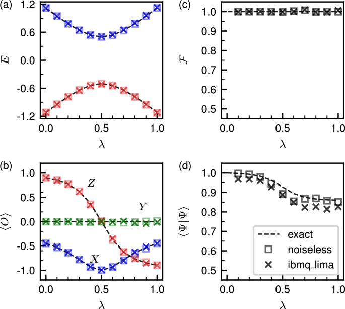
The energy eigenvalues of the ground (red) and the excited state (blue) are plotted in (a). In (b), we plotted (leftlangle Xrightrangle) (blue), (leftlangle Yrightrangle) (green), and (leftlangle Zrightrangle) (red) calculated for the ground states. c, d display the fidelity ({mathcal{F}}) and (leftlangle Psi | Psi rightrangle) for the ground state. In (a–d), dotted lines represent the exact result, boxes represent QZMC results with a noiseless simulator, and crosses represent results with ibmq_lima. In this figure, we used β = 5 and Nν = 400.
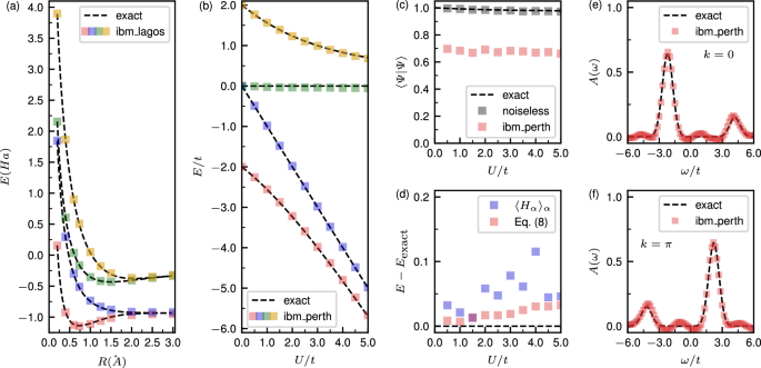
a plots energy eigenvalues of H2 in a STO-3G basis as a function of the bond length. Here, we used β = 5 and NISQ device calculation is conducted with ibm_lagos. In (b–f), we considered the Hubbard dimer. b shows energy eigenvalues as a function of the Coulomb interaction U. In (a) and (b), different states are distinguished by different colors. In (c), we compared (leftlangle Psi | Psi rightrangle) of the ground state calculated with the NISQ device with exact values and noiseless QZMC results. d compares two energy estimators ({leftlangle {H}_{alpha }rightrangle }_{alpha }=leftlangle {Phi }_{alpha }| {H}_{alpha }| {Phi }_{alpha }rightrangle) and Eq. (8). The spectral functions for two different crystal momentum (e) k = 0 and (f) k = π are plotted. For the Hubbard dimer, we used β = 0.5 and ibm_perth is used. In this figure, we used Nν = 100 Monte Carlo samples for each α and the spectral function is calculated with 300 Monte Carlo samples.
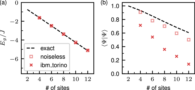
a The energy eigenvalues and (b) (leftlangle Psi | Psi rightrangle) of XXZ model for various sizes from 4 to 12 qubits are plotted. In this figure, dotted lines represent the calculation with exact projection, boxes represent noiselees simulation result, and crosses are QZMC results with the ibm_torino. For QZMC, we used (beta =sqrt{2}), Nα = 1, and Nν = 300.
The one-qubit system results are displayed in Fig. 2. Figure 2a shows the ground and the excited state energy eigenvalues, while Fig. 2b shows ground state expectation value of X, Y and Z operators. Despite device noises in ibmq_lima, measured observables match well with exact values (dashed lines). Moreover, computed ground state fidelity ({{mathcal{F}}}_{alpha }=| langle {Phi }_{alpha }| {Psi }_{alpha }rangle {| }^{2}/langle {Psi }_{alpha }| {Psi }_{alpha }rangle) (Fig. 2c) is almost 1, which demonstrates accurate projection to the desired state by QZMC.
Figure 3 presents computational results for two-qubit systems: H2 and the Hubbard dimer. We determined the energy eigenvalues of H2 within an error of 0.02 Ha using ibm_lagos. Energy eigenvalues for the Hubbard dimer are calculated within an error of 0.06 t on ibm_perth, where t is electron hopping between two hubbard atoms. And we compute the electronic spectral function A(ω)50 of the Hubbard dimer with the NISQ device. Figure 3(e, f) displays A(ω) at k = 0 and k = π, showing good agreements between exact values and measured values.
The additional computations for these one- and two-qubit systems, specifically the parameter dependence of QZMC for the one-qubit system and the ground state energy calculation of the Hubbard dimer with Trotterized time evolution, are provided in Sec. III of the Supplementary Information.
Figure 4 presents the computational results for the XXZ model with 4 to 12 qubits. The energy eigenvalues are well reproduced, even for 12 qubits, despite severe degradation of (leftlangle Psi | Psi rightrangle) due to device noise and trotterization errors. Specifically, we obtained ground state energy errors of 0.015 for 4 qubits, 0.0275 for 6 qubits, 0.016 for 8 qubits, 0.041 for 10 qubits, and 0.051 for 12 qubits on ibm_torino. These values are significantly lower than the errors in (leftlangle Psi | Psi rightrangle) (represented by the differences between the squares and crosses) shown in the right panel of the figure. Thus, we conclude that our method provides reasonable results even in the presence of both device noise and trotterization errors. All calculations were performed with dynamical decoupling (DD)51 and readout error mitigation52, without employing advanced techniques such as zero-noise extrapolation (ZNE)53,54,55 or probabilistic error cancellation (PEC)52,56. We anticipate that larger-scale simulations will become feasible soon with these methods or with advancements in hardware.
Next, we demonstrate our method for a large system by applying QZMC on the Hubbard model at the half-filling in various sizes with noiseless qsim-cirq (https://quantumai.google/qsim) quantum computer simulator. As H0, we choose dimer array, featuring easily implementable non-degenerate ground state. We gradually increased the inter-dimer hopping tinter from 0 to the desired value t as α increased. We explored two geometries, chains and ladders, with periodic boundary conditions, as illustrated in Fig. 5a. For each geometry, we computed systems with 6, 8, and 10 sites when U/t = 5. For QZMC, we used β = 3, with Nα equal to the number of sites and Nν increases as (Vert {H}^{{prime} }{Vert }^{2}) increases. For the time evolution, we used the first order Trotterization28,41,57, adjusting the Trotter steps as system changes. More specifically, we used a maximum of 528 Trotter steps for the 6 × 1 system and up to 1960 steps for the 2 × 5 Hubbard model.

a shows two geometries we considered. Here, colored circles denote sites, solid lines indicate intra-dimer hopping tintra, and dotted lines represent inter-dimer hopping tinter. b displays (leftlangle Psi | Psi rightrangle) for the 2 × 5 Hubbard model as a function of tinter, while (c) presents ground state energy eigenvalues computed from QZMC. In each subplot of (c), red squares denote energies for 6 × 1, 8 × 1, and 10 × 1 models with QZMC, with red dotted lines indicating corresponding exact values. Blue squares and lines represent the same values for 2 × 3, 2 × 4, and 2 × 5 cases. d–g depict the local spectral function for the Hubbard models.
Figure 5c shows that QZMC accurately reproduces the exact ground state energy across various configurations, from 6 to 10 sites, in both chain and ladder geometries. And our method also accurately computes local spectral functions for Hubbard models as shown in in Fig. 5d–g, which reproduces the exact positions and widths of every peak in the spectral functions. Further data not included in Fig. 5(c), such as (leftlangle Psi | Psi rightrangle) for all geometries and spectral functions for the 6-site Hubbard models, can be found in Sec. V of the Supplementary Information.
In Fig. 5, the ground state energies are determined within an error of 0.01t by setting Nα as the number of sites and ({N}_{nu }propto Vert {H}^{{prime} }{Vert }^{2}). Using this parameter rule, we estimate the required number of samples for large-scale Hubbard model simulations. For each α, we compute (leftlangle {Psi }_{alpha }| {Psi }_{alpha }rightrangle), the predictor, and the corrector for the energy difference, using Nν Monte Carlo samples for each quantity. Thus, the total number of required samples is approximately 3NαNν. Since (Vert {H}^{{prime} }Vert) scales linearly with the number of sites, Nν scales quadratically, and the total number of required samples scales cubically. For a 10-site Hubbard chain (ladder), we set Nα = 10 and Nν = 1600 (2594) in Fig. 5, resulting in approximately 4.8 × 10⁴ (7.78 × 10⁴) samples. By applying the cubic scaling derived above, we estimate that a 30-site calculation requires 1.3 × 10⁶ (2.1 × 10⁶) samples, a 50-site calculation requires 6 × 10⁶ (9.73 × 10⁶) samples, and a 100-site calculation requires 4.8 × 10⁷ (7.78 × 10⁷) samples.
Finally, we computed Hubbard chains under open boundary conditions to compare our method with other methods for ground state energy estimation. We compare our method with two state-of-the-art approaches: the Heisenberg-limited method developed by Lin and Tong14, and the quantum complex exponential least squares (QCELS) method developed by Ding and Lin15. We considered three cases: 4 × 1, U = 4; 4 × 1, U = 10; and 8 × 1, U = 10. The initial state (vert {tilde{Phi }}_{0}rangle) was chosen such that (|langle Phi | {tilde{Phi }}_{0}rangle {| }^{2}=0.4), matched the conditions in the references14,15. Both methods were implemented as described in the respective references.
The top panels of Fig. 6 compare the energy estimation error ϵ as a function of the maximum time evolution length T. In most of cases, QZMC requires a shorter T than Lin and Tong’s method and is comparable to QCELS for a precision range of 10−4 to 10−2.

Ground energy estimation errors are shown for: a–c U/t = 4, 4 sites; d–f U/t = 10, 4 sites; and (g–i) U/t = 10, 8 sites. The figures plot the energy estimation error ϵ as a function of (a, d, g) the maximum time evolution length, b, e, h the total number of Trotter steps, and (c, f, i) the total number of samples. In all panels, blue points represent results from the method of Lin and Tong14, black points represent results from QCELS15, and red points represent results from QZMC.
The middle panels show ϵ as a function of the total Trotterization steps NT, which is directly proportional to the circuit depth. In these and the bottom panels, the maximum time evolution length T for each method was set to achieve a similar accuracy of about 0.003 for the exact time evolution. QZMC demonstrates higher precision with fewer Trotterization steps. For example, in the 4 × 1, U/t = 10 case with NT = 412, the error for QZMC is 0.0046, compared to 0.043 for QCELS and 0.015 for Lin and Tong’s method.
The bottom panels plot the total number of samples required for each method. Lin and Tong’s method converges quickly, while QCELS and QZMC converge more slowly, with QZMC requiring the most samples, eventually reaching approximately 105.
In conclusion, overall our method achieves higher precision with shorter circuit depth compared to other state-of-the-art methods, at the cost of requiring more samples. Therefore, QZMC is particularly useful when quantum circuit depth is a limiting factor, but the number of accessible samples is not severely constrained.
In addition to the methods discussed above, our approach can also be compared to adiabatic state preparation (ASP), as both methods follow an adiabatic path. However, QZMC offers two notable advantages over ASP. First, QZMC is resilient to errors such as Trotter errors and device noise, making it more practical in scenarios where such errors are significant. Second, as highlighted in Quantum Zeno Monte Carlo section, QZMC does not require the initial state (vert {Phi }_{0}rangle) to be exact, whereas ASP must begin with an exact (vert {Phi }_{0}rangle). This distinction is important because preparing an arbitrary state on a quantum computer can be exponentially hard34, and the flexibility to start with an approximate initial state enhances the practicality of QZMC. A comparison of ASP and QZMC under the influence of Trotter errors is presented in Sec. V of the Supplementary Information.
Noise resilience of QZMC
Interestingly, our calculational results for observables accurately reproduce exact values even with the device noises (Figs. 2 and 3) and the Trotter errors (Fig. 5). The effect of these noises induces significant deviations of calculated (langle Psi | Psi rangle) (Fig. 2d, 3c, and 5b) from exact values. However, the observable expectation values, which is computed by using the ratio of (leftlangle Psi | O| Psi rightrangle) and (leftlangle Psi | Psi rightrangle) (Eq. (5)) are robust against device noises and Trotter errors. To understand this, we tested the dependence of the calculated observables on the device noise magnitude using the qiskit (https://www.ibm.com/quantum/qiskit) aer simulator. We considered (leftlangle Psi | Psi rightrangle), (leftlangle Psi | Z| Psi rightrangle), and (leftlangle Zrightrangle) of the ground state of the one-qubit system. Figure 7 shows calculational results. As the noise level increases, (leftlangle Psi | Psi rightrangle) decreases and the absolute value of (leftlangle Psi | Z| Psi rightrangle) also decreases (Fig. 7a). Surprisingly, these noise-induced errors cancel each other through the ratio of (leftlangle Psi | Psi rightrangle) and (leftlangle Psi | Z| Psi rightrangle), so that (leftlangle Zrightrangle =leftlangle Psi | Z| Psi rightrangle /leftlangle Psi | Psi rightrangle) (Fig. 7b) remains robust against noise. Since quantum circuits for computing the numerator and denominator are nearly identical, division cancels out common noise effects, making the expectation value resilient. The same argument can be applied to Trotterization (thus, the method is resilient to Trotter error too). Because we use same Trotterization rule for both the numerator and the denominator, common Trotterization errors are canceled out by division. This has been demonstrated numerically in Fig. 8(a, b). In this figure, we computed same quantities considered in Fig. 7 using trotterized time evolutions varying the total trotterization steps NT. We can see that the low-trotterization steps makes (leftlangle Psi | Psi rightrangle) small, but (leftlangle Zrightrangle) does not change a lot because the magnitude of (leftlangle Psi | Z| Psi rightrangle) also decreased by the trotterization.
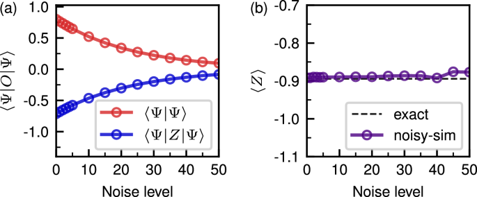
(leftlangle Psi | Psi rightrangle), (leftlangle Psi | Z| Psi rightrangle), and (leftlangle Zrightrangle) of the one-qubit system considered in the Fig. 2 is drawn as a function of the noise level. The calculations are conducted with the qiskit noisy simulator using the noise model of ibmq_lima. In this figure, we used Nα = 10, β = 5 and Nν = 400.
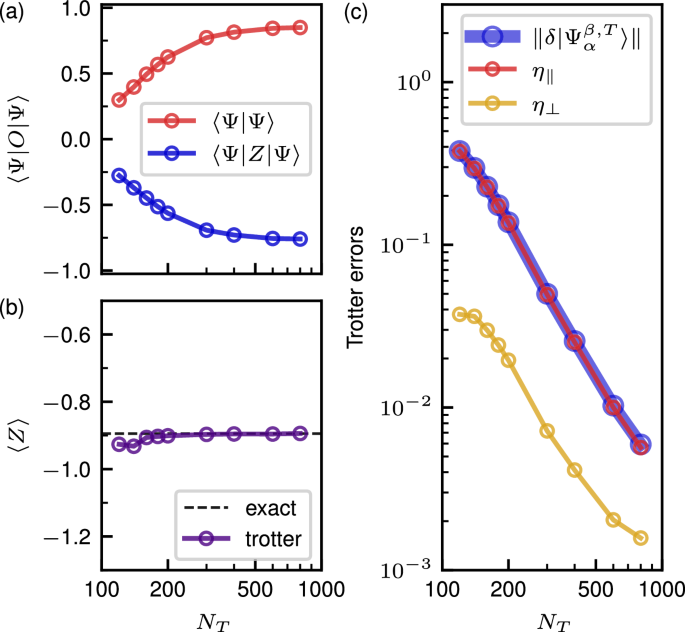
a, b show (leftlangle Psi | Psi rightrangle), (leftlangle Psi | Z| Psi rightrangle), and (leftlangle Zrightrangle) as functions of the total number of Trotter steps, for the one-qubit system considered in Fig. 2. In (a, b), Nν = 400 was used. c displays the total Trotter error (| leftvert delta {Psi }_{alpha }^{beta ,T}rightrangle |), the parallel component η∥, and the orthogonal component η⊥, plotted against the total number of Trotter steps. For (c), Nν = 4000 was used to reduce the statistical error. In all panels, we set Nα = 10 and β = 5.
Figures 7 and 8a, b demonstrates that error cancellation through division occurs in practice for both device noise and Trotter errors. However, since these errors arise from fundamentally different sources, the mechanisms behind their cancellation differ. In following, we provide a detailed analysis of how error cancellation occurs for each type of error and additional notes.
First, we discuss the mechanism for the device’s noise resilience. In our method, we measure consecutive time evolution using a single ancilla qubit (See Sec. II D 2 of the Supplementary Information for quantum circuits). With this in mind, let’s examine the following simple example. Consider a qubit with the density matrix ρ. Then, exact outcome of a Z measurement on this qubit is given by ({rm{Tr}}(rho Z)). The effect of noise the qubit can be described as ({mathcal{E}}(rho ))3. With this noise, the outcome of the Z measurement becomes ({rm{Tr}}({mathcal{E}}(rho )Z)). Consider the depolarizing channel as a specific type of noise, which alters the state ρ to ({mathcal{E}}(rho )=pI/2+(1-p)rho). Here, p represents the probability of depolarization. With this model, ({rm{Tr}}({mathcal{E}}(rho )Z)) becomes ((1-p){rm{Tr}}(rho Z)). Now, imagine another qubit with the density matrix ({rho }^{{prime} }) subjected to the same noise channel. The Z measurement of this qubit yields ((1-p){rm{Tr}}({rho }^{{prime} }Z)). Then, the ratio of the measurement outcomes of two qubits with noise channel is
which is same with the exact value. This demonstrates that the effect noise can be effectively canceled out by the division. Though we only showed the case with the depolarizing channel, same cancellation occurs for bit and phase flip channels. Similar discussion can also be found in the literature on the quantum-classical hybrid Quantum Monte Carlo algorithm (QC-QMC)58, which estimates the wave function overlap efficiently using shadow tomography.
To analyze the resilience of QZMC to Trotter errors, we consider the state
as defined in Error analysis of (langle {Psi }_{alpha }^{beta }| {Psi }_{alpha }^{beta }rangle) section. The error term (vert delta {Psi }_{alpha }^{beta ,T}rangle) can be decomposed into two components: one parallel to (vert {Psi }_{alpha }^{beta }rangle) and the other orthogonal to it. Suppose the error consists only of the parallel component. In this case, we can express the state as
Here, η∥ represents the norm of the parallel error, and ϕ∥ is the associated phase shift. In such a scenario, the expectation value of an observable O is
Thus, the parallel component of the error cancels out through division, demonstrating that QZMC is inherently resilient to this type of Trotter error.
In practice, however, the error also contains an orthogonal component ({eta }_{perp }vert {Psi }_{alpha ,perp }^{beta }rangle), resulting in
Here, η⊥ denotes the norm of the orthogonal component and (vert {Psi }_{alpha ,perp }^{beta }rangle) is a normalized vector orthogonal to (vert {Psi }_{alpha }^{beta }rangle). Unlike the parallel component, the orthogonal error does not cancel out through division. Therefore, the key to Trotter error resilience lies in the relative magnitudes of η∥ and η⊥. Numerical tests in Fig. 8(c) demonstrate that η⊥ ≪ η∥ in practice. This dominance of the parallel component ensures that error cancellation through division remains effective, making the method robust against Trotter errors.
One notable point regarding noise resilience is that, in addition to the noise cancellation effect demonstrated in Figs. 7, 8, the use of the estimator in Eq. (8) enhances robustness against noise. This is because it computes only energy differences, limiting the influence of noise to the energy difference Eα − Eα−1. Figure 3(d) shows this. In this figure, we can see that the energy computed by Eq. (8) is more precise and stable compared to the energy computed by ({leftlangle {H}_{alpha }rightrangle }_{alpha }=leftlangle {Phi }_{alpha }| {H}_{alpha }| {Phi }_{alpha }rightrangle) using Eq. (5).
Another important note is that our discussion on noise resilience does not imply resilience to statistical noise. In fact, as the noise level increases, the impact of statistical error on the results is amplified, requiring a larger number of samples. More specifically, device and Trotter errors reduce (leftlangle {Psi }_{alpha }| {Psi }_{alpha }rightrangle), which appears in the denominator of our observable estimators. Because the statistical error of the energy estimator is proportional to (see Eq. (S.48) of the Supplementary Information for the explicit form)
if (leftlangle {Psi }_{alpha }| {Psi }_{alpha }rightrangle) is reduced to ((1-p)leftlangle {Psi }_{alpha }| {Psi }_{alpha }rightrangle), the statistical error amplification factor is
For example, if device or Trotter errors reduce (leftlangle {Psi }_{alpha }| {Psi }_{alpha }rightrangle) from its exact value of 0.8 to half of that value, the statistical error is amplified by a factor of approximately 3.36.
Discussion
In this work, we introduced the quantum Zeno Monte Carlo (QZMC) for the emerging stepping stone era of quantum computing13. This method computes static and dynamical observables of gapped quantum systems within a polynomial quantum time, without the need for variational parameters. Leveraging the Quantum Zeno effect, we progressively approach the unknown eigenstate from the readily solvable Hamiltonian’s eigenstate. This aspect distinguishes our method from other methods for phase estimations, which necessitate an initial state with significant overlap with the desired eigenstate5,6,14,15,25,26,59. Preparing a state with substantial overlap with an eigenstate of an easily solvable Hamiltonian is much simpler than preparing an initial state with non-trivial overlap with the unknown eigenstate, making our algorithm highly practical compared to other methods. The next characteristic of the algorithm is its computation of eigenstate properties by dividing the properties of the unnormalized eigenstate by its norm squared (Eq. (5)). We demonstrated that this approach effectively cancels out noise effects in the denominator and the numerator, rendering the method resilient to device noise as well as Trotter error. This resilience arises from the similar noise levels experienced by both the denominator and the numerator of observable expectation value, leading us to conclude that our approach is well-suited for homogeneous parallel quantum computing.
Methods
NISQ simulation
Here, we provide the details of the NISQ simulations in Figs. 2–4. Throughout the simulations, we used Ns = 4000 shots for one- and two-qubit systems, and Ns = 2048 shots for the XXZ model. Since any 1- or 2-qubit unitary operation can be represented with a small number of gates60, the consecutive time evolutions encountered in QZMC can be implemented within a shallow circuit with a few parameters. For the 1-qubit system, the parameters θ1, θ2, θ3, θ4 for the unitary matrix U are obtained from60:
For the 2-qubit system, we applied the two-qubit Weyl decomposition61, as implemented in Qiskit.
For the XXZ model, we set (beta =sqrt{2}) and combined ({({P}_{1}^{beta })}^{2}) in Eq. (8) into a single integral. For Trotterization, we employed second-order Trotterization based on the efficient implementation of Trotterized quantum circuits49, using two Trotter steps. We begin with XXZ dimers, described by the Hamiltonian
For systems with up to 8 qubits, we used the first-order perturbation energy as a predictor for the energy. For the 10-qubit system, we employed E2 + E8 as the predictor, where E2 is the energy of a single XXZ dimer, and E8 is the energy of an 8-site XXZ model computed using ibm_torino. Subsequently, using the computed E10, we used E2 + E10 as the predictor for the 12-site XXZ model. We used an initialization circuit that prepares the vacuum state (leftvert {0}^{n}rightrangle) when the ancilla qubit is in (leftvert 0rightrangle), and the ground state of H0 when the ancilla qubit is in (leftvert 1rightrangle). The specific initialization circuit for the 10-site XXZ model is provided in the Supplementary Information. The number of gates used in this simulation, in terms of the basis gates of ibm_torino, is 237 for 4 sites, 384 for 6 sites, 534 for 8 sites, 696 for 10 sites, and 857 for 12 sites.
Noiseless simulation
Here, we discuss more detailed information about noiseless simulations (Figs. 5, 6). In these calculations, we consider the Hubbard model which is described by the Hamiltonian
with the chemical potential μ = U/2, corresponding to the half-filling. The first two terms represent the kinetic energy and are denoted as Ht, while the last term represents electron-electron interaction and is referred to as HU. The ground state of the Hubbard dimer can be expressed as
Here, the angle θd is given by
The ground state of H0, composed of a collection of dimers, is formed by the direct product of Eq. (35) for each dimer. The following describes the details specific to the calculations in Fig. 5, performed using the cirq quantum computer simulator. In the simulations, we used Nν and Trotter steps (NT) that varied with the system size, while fixing the number of shots at Ns = 10, 000. Based on Eq. (22), Nν was set proportional to (Vert {H}^{{prime} }{Vert }^{2}), where
and
The proportionality constant was determined by testing the 6 × 1 system numerically. The first-order Trotterized time evolution U1(τ) for the Hubbard model with nT Trotter steps introduces a Trotter error41 given by
where
Since all orbital indices are equivalent, (Vert [{c}_{isigma }^{dagger }{c}_{jsigma },{sum }_{i}{n}_{iuparrow }{n}_{idownarrow }]Vert) remain constant for any i and j. Consequently,
where Nintra denotes the number of intra-dimer hoppings and Ninter represents the number of inter-dimer hoppings, and C is a proportionality constant.
Based on this, NT,α was determined as
with a minimum value of 20. Specific values of Nν and total Trotter steps ({N}_{T}=2mathop{sum }nolimits_{alpha = 1}^{{N}_{alpha }}{N}_{T,alpha }) for each model are summarized in Supplementary information.
Next, we provide detailed information on the comparative study for the Hubbard models in Fig. 6. In this case, we considered open boundary conditions, and the initial state is prepared from direct product of Eq. (35), with θd adjusted to achieve (| leftlangle Phi | {tilde{Phi }}_{0}rightrangle {| }^{2}=0.4).
For all data in Fig. 6, each calculation is repeated 30 times, and the absolute values of energy errors were averaged over repetitions. To measure the maximum time length T, we used the 99th percentile of the distribution of time evolution lengths, as all three methods are stochastic. This means that 99% of the time evolution lengths are smaller than T.
The computational parameters are set according to the references for the compared methods. For Lin and Tong’s method14, we set the parameter δ = 4/d as in the reference and varied d, which determines the time length. We used 1800 samples, consistent with the original paper. For QCELS15, we followed the relative gap D estimation and parameter settings in the original article, using d = ⌊15/D⌋ and N = 5. The sample number for each nτj was set to 2048, higher than the values used in the original paper.
For QZMC, we used Nν = 16,384 for calculations with ϵ ≥ 0.001 and Nν = 1,638,400 for calculations with ϵ < 0.001. For precise calculation, after obtaining the energy difference using Eq. (8), we recomputed it with the obtained Eα value at each α.
For the middle and bottom panels of Fig. 6, we noted that the maximum time evolution length T is set for each method to achieve a precision ϵ of about 0.003 under exact time evolution. In practice, the following parameters were used in our calculations.
For the 4-site Hubbard model with U/t = 4, we used d = 4000 for Lin and Tong’s method, resulting in T = 398.56 and ϵ = 2.46 × 10⁻³. For QCELS, we used J = 5 and τJ = 40, yielding T = 23.09 and ϵ = 2.45 × 10⁻³. In QZMC, we used β = 1.6, which gave T = 20.53 and ϵ = 2.23 × 10⁻³.
For the 4-site Hubbard model with U/t = 10, we used d = 6000 for Lin and Tong’s method, leading to T = 323.26 and ϵ = 2.79 × 10⁻³. In QCELS, we used J = 7 and τJ = 108, resulting in T = 32.32 and ϵ = 3.16 × 10⁻³. For QZMC, we used β = 2.6, yielding T = 33.36 and ϵ = 3.24 × 10⁻³.
For the 8-site Hubbard model with U/t = 10, we used d = 12000 for Lin and Tong’s method, producing T = 316.13 and ϵ = 2.84 × 10⁻³. In QCELS, we used J = 9 and τJ = 372, resulting in T = 54.65 and ϵ = 2.42 × 10⁻³. For QZMC, we used β = 4.2, giving T = 53.88 and ϵ = 2.96 × 10⁻³.
In the Trotterization tests, first-order Trotterization was employed for all methods. In QZMC, the Trotter steps NT,α for each α were determined as
and the total Trotter steps NT were computed as 2∑αNT,α. For calculations in Fig. 6, we used a shot number Ns = 2048.


Responses