Rapid evolution of energetic lightning strokes in Mediterranean winter storms

Introduction
The global distribution of winter lightning provided by the World Wide Lightning Location Network (WWLLN)1 shows three areas with an enhanced lightning activity in the northern hemisphere: the lightning density exceeds 0.01 strokes per kilometer square per year only in the eastern part of North America, in the Mediterranean basin and in Japan2. In winter clouds, microphysics and electrification are different from summer thunderclouds. The main difficulty for the winter thundercloud to be formed is a lack of sufficient amount of water vapor because of low ambient temperatures. That is why the “cold air over warm water” scenario for development of winter thunderclouds was proposed3. The three areas in the northern hemisphere, which are being most frequently hit by winter lightning, clearly fit this scenario. The warm Sea of Japan is overrun by cold winds from Siberia, producing numerous thunderstorms at the western coast of Japan. The Great Lakes in the US are overblown by arctic winds arriving from Canada, which leads to an increased amount of winter storms in the northeastern part of the US. In Europe, the cold air masses coming from the low-pressure systems developed above the Atlantic Ocean often stagnate above the warm Mediterranean Sea, which results in significant winter lightning activity. In spite of the fact that the scenario for development of winter thunderclouds is the same for all above-mentioned regions, the thundercloud properties significantly differ. Unlike the winter thunderclouds in the Mediterranean, the Japanese ones are tilted, their tops reach lower altitudes, the cloud base is located closer to the surface, and the charge structure is different as well4. While Mediterranean winter thunderclouds exhibit either a normal or an inverted tripole charge structure5, Japanese winter clouds display all types of charge structures, including positive or negative dipole charge arrangements. The horizontal extent of the Japanese thunderclouds is much larger than the vertical extent. Due to the thundercloud tilt, the charge structure is asymmetrical, likely contributing to a high percentage of positive lightning6.
The winter thunderclouds differ substantially from these occurring in summer. The 0°-isotherm decreases near to the Earth surface, the ascent speed of ice crystals at 1–2 km altitude is only 1 m/s or less3. The regions of opposite charge are usually separated by only 1–2 km and the Convective Available Potential Energy (CAPE) is one order of magnitude lower in winter7.
The winter lightning occurring in Japan has been studied by many researchers, and lightning characteristics are well documented8,9,10,11,12,13,14,15,16. The properties of winter lightning occurring at the Northeast of US were described in several studies17,18,19. The Mediterranean thunderstorm climatology shows that winter thunderstorms are less frequent than the summer ones, but on average, cover twice large area, propagate faster, and predominantly take place over the maritime areas20. Statistical analysis of lightning strokes occurring in the Mediterranean area21 reports the largest current intensities in January, over sea and during nighttime. Based on the altitude distribution of intracloud (IC) discharges, the authors found that the cumulonimbus clouds are the least vertically developed in winter. The lightning activity was found to be positively related to the sea surface temperatures, especially during colder months when lightning activity concentrates above the water22. The lightning activity in the Eastern Mediterranean occurs exclusively in winter and was found to be the most intense along the coast plain23. Other studies were focusing on the relation between lightning and rainfall in the Mediterranean winter storms24 or on the properties of winter sprites25,26, nevertheless, a detailed investigation of electromagnetic signatures of winter lightning in this region is still missing.
The characteristics of winter lightning considerably differ from those of summer lightning. Firstly, the lightning discharges are occurring mostly above the water2. Secondly, there is usually a higher percentage of positive cloud-to-ground (CG) lightning during winter27, reaching 30% in Mediterranean, while in summer there is about 10% of positive CG lightning28. Thirdly, the currents flowing in the winter lightning channels belonging to negative strokes reach on average larger peak values than their summer counterparts29. There is even a hypothesis, that the global enhancement of the negative peak currents above the oceans likely originates in the observations of larger peak current values reported during winter storms30. In winter, a reduced amount of lifted water vapor may hypothetically result in the absence of larger water droplets in the cloud’s mixed-phase region. Consequently, conductivity in this region decreases, the breakdown field increases, and the average peak currents tend to rise18. Fourthly, the lightning evolution period defined in the electromagnetic recordings as the time interval from the first preliminary breakdown (PB) pulse to the return stroke (RS) pulse31, was reported to be very short during winter in Japan12,13,14 and in the US18.
The preliminary breakdown phase of lightning discharges has been already studied for several decades by many groups of researchers31,32,33,34,35,36,37,38. This phase of lightning evolution is very well recognizable in electromagnetic recordings as a group of approximately regularly distributed bipolar pulses. These PB pulses—also known as initial breakdown (IB) pulses—are believed to be present in the recordings of electromagnetic signals emitted just after the initiation of all cloud-to-ground (CG) or intra-cloud (IC) lightning discharges32. A bidirectional leader is propagating in the developing lightning channel during the PB phase. The pulses are electromagnetic signatures of sudden elongations of the initial negative leader in the ambient thunderstorm electric field. The waveform characteristics of recorded PB pulses are believed to reflect directly the properties of the leader (for example a step length and the line conductivity of the channel) and the amplitude of the electric field inside the thundercloud39. The peak amplitudes of pulses can be comparable to those of the RS pulses, indicating that the in-cloud currents can reach several tens of kilo-amperes37,40,41,42.
The PB pulses can be categorized based on their duration and bipolarity. The “classical” PB pulses are defined as bipolar pulses with a total pulse duration from 10 to 100 µs43,44. The narrow PB pulses are defined as bipolar or unipolar pulses narrower than 10 µs. The classical PB pulses were found to be stronger than the narrow PB pulses: usually, the amplitudes of classical PB pulses exceed 25% of the amplitude of the largest pulse in the train43. Optical measurements45 revealed that the classical PB pulses are generated by the currents flowing in the elongating vertical channels. Many narrower, mainly unipolar pulses occur between the classical PB pulses43. They can occur both before and after the largest PB pulse. The pulses narrower than 4 µs were found to represent 57–98% of all pulses in the PB trains43. These narrower pulses were probably generated by small currents during a minor prolongation of the in-cloud lightning channel. There are often subpulses observed on the rising or falling edges of classical PB pulses. These subpulses are considered to be signatures of connecting branches to the main in cloud leader channel and their presence indicates a corresponding increase of the current46,47. The studies of lightning initiation phase focus nearly exclusively on the classical PB pulses32,33,34,35,36,37.
There are two main parameters that the majority of studies analyzing the electromagnetic signals emitted by CG lightning discharges provide. The first parameter, relevant to the velocity of the discharge evolution, is the time interval between the first PB pulse and the RS pulse (PBP-RS). The PBP-RS parameter reflects the properties of the thundercloud and associated electric fields and is used to investigate differences in lightning initiation processes across various regions and seasons. The PBP-RS time interval ranges from a fraction of a millisecond to one-tenth of a second48. In the case of strong negative strokes, this parameter is primarily influenced by the properties of downward negative leaders and serves as an input for modeling the leaders in lightning protection studies49,50. The second parameter is the amplitude ratio of the largest PB pulse to the RS pulse (PBP/RS), which indicates the strength of the charge centers in the bottom thundercloud dipole. This parameter is usually below one but can reach values as high as five48.
Since the presence of PB pulse trains serves as an indicator for lightning initiation, broadband recordings can be effectively integrated with data from narrowband arrays to comprehensively interpret very high frequency (VHF) measurements36,51,52. The PB pulses were found to carry very large charges from −0.12 C to −1.7 C44 and thus fundamentally differ from the stepped leaders which carry charges smaller by 3–5 orders of magnitude53. The amplitudes of PB pulses, the length of the PB trains, and the PB interpulse amplitudes are being often analyzed and modeled to infer thundercloud properties, the electric fields inside thunderclouds or to estimate the currents flowing in the in-cloud lightning channels just after the lightning initiation using the easily accessible electromagnetic measurements39,44,46,54,55,56. The unified engineering model of the first stroke in downward negative lightning57 introduced an amplitude envelope for a PB pulse train, during which the pulse amplitudes increase up to the largest pulse and then decrease again. Such envelope is considered to reflect the basic simple tripolar thundercloud structure. The initial negative leader starts between the main negative and lower positive charge centers, and after its initiation, it propagates downward in a stepwise manner. The tip of the negative leader is attracted by the positive charge center and the pulse amplitudes increase. Whenever it reaches the lower positive charge center and propagates through it towards the thundercloud base, the amplitudes decrease.
Very rarely, Narrow Bipolar Events (NBEs) are found to precede the first PB pulse of the negative CG flash58 in the electromagnetic recordings. The NBEs are impulsive and powerful intracloud discharges, which are usually observed in isolation or starting an IC flash59. The NBEs can be distinguished from the classical PB pulse by an abrupt onset of the pulse and a pulse full-width at half-maximum (FWHM) of about a few microseconds only60,61.In this study, we investigate the initiation phase of winter lightning in the West Mediterranean. We focus on energetic strokes with peak currents exceeding 100 kA. We cannot classify all of them as superbolts by definition, as this term specifically refers to strokes radiating three orders of magnitude more energy than an average stroke62 and an average Mediterranean winter stroke has a peak current of approximately 20 kA5,21. Our study was strongly driven by the specific needs of lightning location systems (LLS)28 for several reasons.
a) High peak current RSs are challenging for the LLS operators to detect, as they are relatively rare. Nevertheless, their occurrence is increasing, especially in winter and the associated damages can be significant, particularly over land.
b) Estimating high peak currents, which is essential for lightning protection specifications, poses a challenge for LLS. High peak current discharges have not been observed in triggered lightning experiments, which prevents the calibration of the Transmission Line Model typically used to convert radiated fields into peak currents63.
c) Intense electromagnetic PB pulses are sometimes misclassified as +CGs, and RS pulses with atypical shapes associated with high peak current strokes are occasionally discarded by automated LLS procedures.
We introduce the instrumentation and the dataset of waveform snapshots (see the Methods section), we examine the properties of PB pulse trains preceding strong negative CG flashes and inspect the distribution and time evolution of the pulse peak amplitudes and interpulse intervals, and, finally, we discuss our results.
Results
Electromagnetic characteristics of selected energetic winter strokes as a function of the peak current
The map in Fig. 1a shows the spatial distribution of energetic negative CG lightning (with peak currents stronger than −100 kA) in our data set, with a more prevalent occurrence of lightning above the seawater. The histogram in Fig. 1b displays the distribution of peak currents as estimated by MÉTÉORAGE. The median value of the peak current of strokes used in our study was −135 kA, two reported peak currents exceeded −300 kA.

a Locations of lightning strokes included in our study. The position of the receiving station is shown by a black asterisk. b Distribution of peak currents of the analyzed lighting discharges.
Examples of magnetic field waveforms emitted by lightning strokes included in our study are shown in Fig. 2. The locations of the causative RSs belonging to the examples from Fig. 2a–c are identified in the map in Fig. 1a by black arrows. The waveform in Fig. 2a was recorded on 30 November 2014 at 14:56:23.3829UTC and consists of following lightning phases: a PB pulse train delimited by a red shading, an intermediate stage (IS) is marked by a gray shading, a stepped leader (SL) marked by a green shading, and a RS pulse. Because of a presence of an intermediate stage defined as a time interval between the PB and SL stages without a significant pulse activity12,64,65, the lightning evolution from the first PB pulse to RS pulse (PBP-RS) lasted 3.4 ms. The ratio between the largest PB pulse peak amplitude and the RS pulse peak amplitude (PBP/RS) was 0.14. The waveform in Fig. 2b, which was recorded on 16 December 2014 at 03:49:50.3378UTC clearly lacks the intermediate stage, and the PB pulse train and the stepped leader joined each other or even intermingled just before the RS pulse. This lightning evolved very fast, the PBP-RS duration was only 0.7 ms, the largest PB pulse was five times smaller than the RS pulse. The transition between the PB phase and the SL phase is not well determinable, the PB pulses and the SL pulses overlap. From our data set, only 14 events exhibit a clear intermediate stage, and 25 events seem to lack the SL pulses at all. As the SL pulses are emitted by a discharge propagating below the cloud base in a stepped manner with a step length of about 50 m48, the absence of SL pulses might indicate that the bottom of the thundercloud was very close to the surface. It is also possible that the SL pulses were not clearly recognizable in our records being mixed with the pulses produced by the incloud leaders propagating in branches, which typically appear in the late stages of negative CG flashes48.
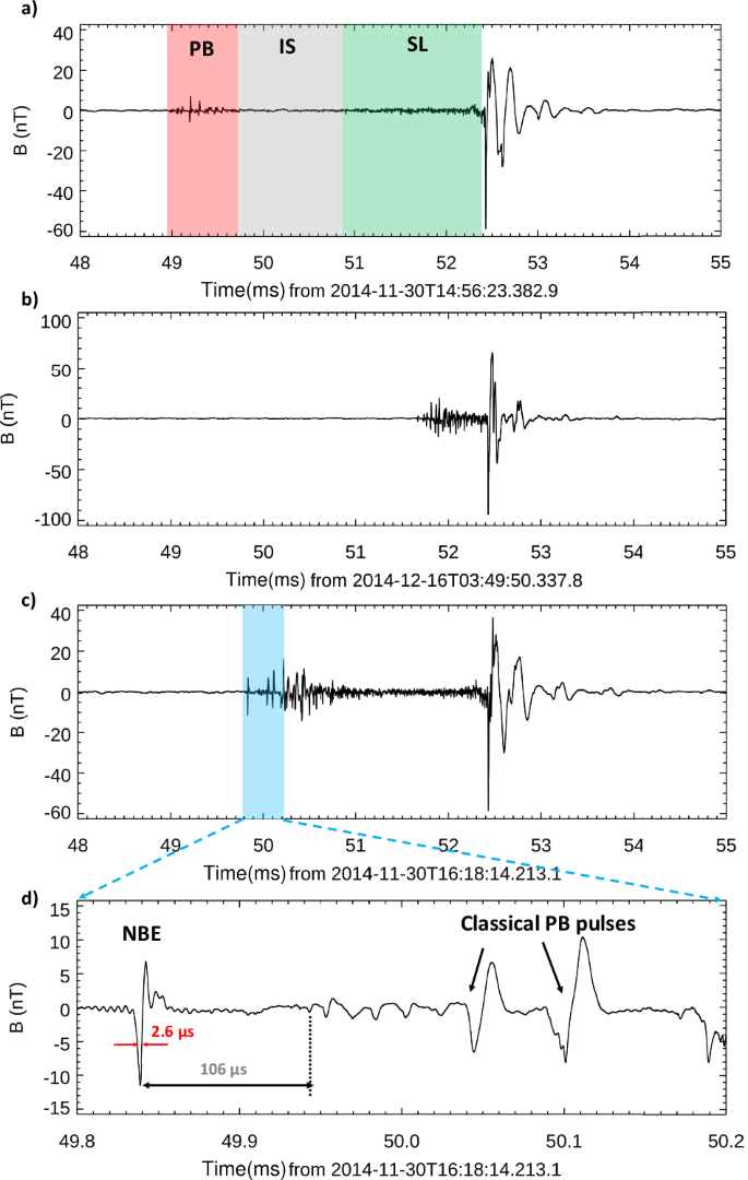
a The waveform emitted by the discharge with PBP-RS separation of 3.4 ms, a peak current of −193 kA, recorded on 30 November 2014 UTC at 14:56:23.3829. Individual parts of the pre-stroke activity are indicated by colored boxes: Preliminary Breakdown phase in red, an Intermediate Stage (IS) in gray, a stepped leader in green. b The waveform emitted by the discharge with a short PBP-RS separation of 760 µs, a peak current of −198 kA, recorded on 16 December 2014 UTC at 03:49:50.3378. c The waveform emitted by the discharge starts with a Narrow Bipolar Event occurring 106 μs before the PB pulse train. The causative discharge was recorded on 30 November 2014 UTC at 16:18:14.2131. The peak current was estimated to be −139 kA by MÉTÉORAGE. d A detailed view at the NBE pulse and the beginning of the PB train.
We observed also six untypical PB trains which started by a larger pulse belonging to a Narrow Bipolar Event (NBE) preceding the first regular PB pulse. The NBE pulses were not always the largest pulses in the pre-stroke period. The time delay of the first PB pulse after the NBE pulse varied from 47 to 106 µs. The detailed view on the event with the largest time delay of 106 µs is available in Fig. 2c and d. The FWHM of the NBE pulse is 2.6 µs, typical for NBEs60,61 and narrower than following classical PBPs with a typical FWHM of a few tens of µs as can be seen in Fig. 2d.
The histograms in Fig. 3a, b respectively show the distribution of the PBP-RS time separation (the time between the first PB pulse exceeding the noise threshold of 0.5 nT and the RS pulse), and the distribution of the PBP/RS amplitude ratio (the amplitude ratio between the largest PB pulse and the RS pulse). These two important properties reflect the specificity of the winter negative lightning discharges. The duration of the lightning evolution is on average much shorter than for an average negative lightning, which is a few tens of milliseconds32. In the case of the analyzed Mediterranean winter lightning discharges we obtain a duration of 1.70 ± 0.94 ms (with a median value of 1.5 ms), varying from an extremely short value of 220 μs to 6 ms. If the very first PB pulses were exceptionally obscured by background noise, the PBP-RS time interval may be underestimated by a delay corresponding to the typical interpulse interval. However, this PBP-RS error of a few tens of microseconds is negligible in most cases. The peak amplitude of the largest PB pulse for average negative lightning reaches 20–50%32,66; in our data set this ratio reaches one-quarter of the RS pulse amplitude (0.24 ± 0.13). Note, that in case of events with non-separable PB and SL phase or even missing clear SL phase we used the largest pre-stroke pulse to estimate the PB/RS ratio. In majority of events this largest pre-stroke pulse occurred within the first millisecond after the lightning initiation, as shown in Fig. 3c. Nevertheless, there were events with the largest pulses occurring surprisingly very close to the corresponding RS pulses, as seen, for example, in Fig. 3d.
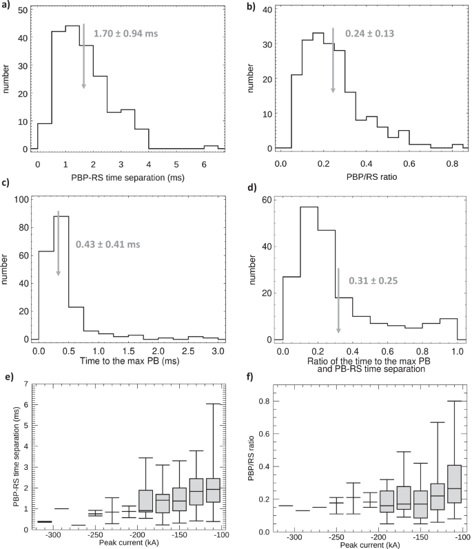
a Distribution of PBP-RS time separations. b Distribution of ratio of PBP/RS amplitudes. c Distribution of the time intervals needed to achieve the largest PB pulse. d The distribution of the position of the largest PB pulse in respect to the first PB pulse in the train. e PBP-RS time separation and (f) PBP/RS ratio as a function of the peak current displayed in box and whisker plots showing minimum, median, and maximum values. For currents weaker than −200 kA we show also the first and third quartiles by shaded rectangles.
To understand the relation of PB parameters to the corresponding large peak current, we divided the data set in 20 kA bins and displayed it as boxplots in Fig. 3e, f. For peak currents weaker than −200 kA the shaded boxes go from the first quartile to the third quartile. Horizontal lines going through the boxes show the median value. The whiskers go to the minimum and maximum. For peak currents stronger than −200 kA (15 events) the number of cases in a bin is lower than five, and we display only the minimum, median, and maximum values.
We performed a similar analysis also for the set of negative lighting strokes with peak currents weaker than −100 kA detected during the same winter campaign. The peak currents were nearly equally distributed between −5 and −100 kA (Fig. S1a). The parameter PBP-RS was on average 5.20 ± 7.79 ms, while the mean value of the parameter PBP/RS was 0.63 ± 0.74. The distribution of these two parameters describing the waveforms from the lightning initiation up to the RS pulse together with their relation to the peak current are displayed in Fig. S1b–e.
Distribution of amplitudes and interpulse intervals within the pre-stroke period
As we are unable to estimate the boundary between the PB pulses and stepped leader pulses in the majority of events, we decided to investigate the properties of all pulses appearing up to the RS pulse. When visually inspecting the waveforms at the beginning of the pre-stroke period, we recognize significant differences in the shapes of the envelopes formed by the larger pulse peaks. In majority of events (73%) the pulse train started with smaller pulses and the largest PB pulse occurred later towards the middle of the train and the pulse envelope shape could resemble a diamond or a half of it (examples in Fig. 4a, b, marked by blue shading). In a few cases, the largest PB pulse appeared at the beginning of the train (3% of events). We noted also six untypical trains which started by pulses belonging to NBEs (Fig. 4c and another example in detail in Fig. 2c, d). In the remaining 24% of cases, the pulses are somewhat randomly distributed (Fig. 4d). The distribution of PB pulse envelope shapes for the set of 291 negative discharges from the same winter campaign but with peak currents weaker than −100 kA was very different. 75% of PB trains were composed of irregularly distributed pulses, 24% of envelopes resembled a diamond or half of it and 1% of pulse envelopes began with the largest PB pulse. We also found five untypical trains starting with pulses belonging to NBEs. All trains, which formed envelope patterns described above, were often followed by irregularly distributed pulses toward the return stroke pulse.
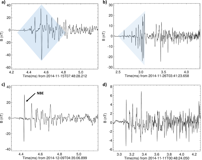
a Example of a “diamond” shape pattern belonging to the waveform recorded on 15 November 2014 at 07:48:28.212UTC. b Example of a train with increasing PB pulse amplitudes at the beginning of the train (“half diamond” shape) belonging to the waveform recorded on 26 November 2014 at 03:41:23.658UTC. c Example of a train starting with an NBE pulse occurring at the beginning of the train belonging to the waveform recorded on 9 December 2014 at 04:35:06.899UTC. d Example of a train with randomly distributed pulses belonging to the waveform recorded on 11 November 2014 at 00:48:24.050UTC. Blue shading in (a, b) represents shapes as seen by human eyes focusing on the largest pulses only.
To investigate the distribution and time evolution of peak amplitudes of pre-stroke pulses and interpulse intervals during the evolution of the strong winter discharges in detail, we determined the times and the peak values of individual pulses. The semi-automated method for obtaining the pulse peaks consisted of three steps.
1) From each waveform, we removed the RS pulse and normalized the remaining part by the peak amplitude of the largest pulse within the pre-stroke period.
2) We chose a minimum time separation of 10 μs between individual peaks and we removed the peaks with a closer separation from the analyzed dataset. This value was set to capture the majority of classical PB pulses defined as bipolar pulses with a total duration larger than approximately 10 µs43,44,48 and exclude shorter and weaker unipolar pulses. By this limitation, we also exclude subpulses, which are believed to be produced by small connecting branches47 and whose amplitude cannot be obtained by our automated procedure. The resulting set of peak amplitudes marked by blue crosses in the individual waveforms shown in the Fig. S2.
3) The initial polarity of the PB pulses in the waveforms depended not only on the polarity of the current but also on the angle between the normal vector to the antenna loop plane and the antenna-discharge separation vector. For the following analysis, we unified the dataset by inverting the sign of a subset of the waveforms, in order to ensure that the leading part of each bipolar PB pulse peak always exhibits positive polarity, while the immediately following opposite overshoot consistently displays negative polarity. Next, we used a threshold of 5% of the largest pre-stroke pulse peak amplitude to select the local maxima and minima for peak values. The threshold was established for practical reasons, to allow comparing the pulses belonging to individual events using the worst-case background noise level as a basis.
The results of the employed automated procedure were manually checked. The dataset consists of 9034 pairs of normalized pulse peak amplitudes and their time of occurrence and 8271 pairs of amplitudes and times of the normalized opposite polarity pulse peaks. The distribution of all pre-stroke relative pulse peak amplitudes exceeding 5% of the largest pre-stroke pulses is plotted for the initial polarity pulses (the same as the polarity of the RS peak) in Fig. 5a.
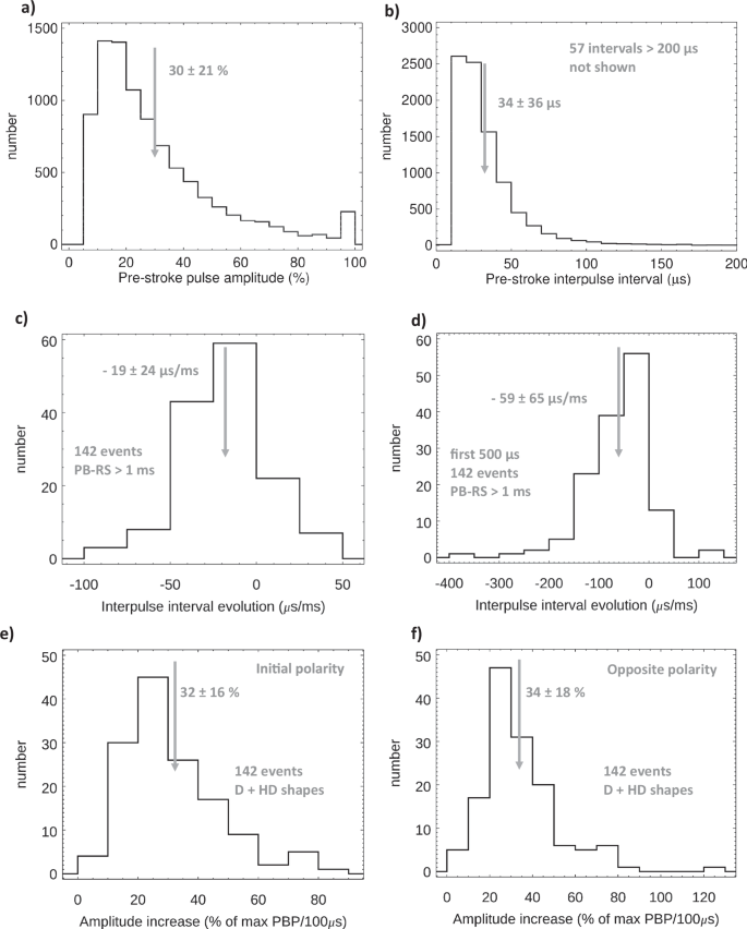
a Distribution of the pulse peak amplitudes relative to the max pulse. b Distribution of the inter-pulse intervals. Interpulse intervals evolution in the first (c) 1 ms and (d) 500 μs from the discharge initiation. Increase of the pulse peak amplitudes within the pulse trains with the diamond and half diamond shapes for (e) the initial and (f) opposite pulse polarities.
Similarly, we show the distribution of all interpulse intervals (time intervals between the peaks of neighboring pulses with peak amplitudes exceeding 5% of the peak amplitude of the largest pre-stroke pulse) above 10 μs for the initial polarity of the bipolar pulses in Fig. 5b. This histogram is limited to 200 μs, nevertheless there are 57 interpulse intervals exceeding this value. The longest interpulse interval reached 1.2 ms. Most of these outliers belong to the pre-stroke processes with the intermediate stage (example in Fig. 2a) with very weak or absent pulses and these large interpulse intervals represent the time delay between the end of the PB pulse train and the beginning of the stepped leader. The same histograms for the opposite polarity pulses (not shown) are very similar.
To estimate the evolution of the interpulse intervals we selected 142 events with PBP-RS time intervals longer than 1 ms. We calculated the interpulse intervals and linear trends to quantify their evolution. Within most trains, the gaps between the pulses were smaller toward the end of the train. Within 29 trains, we found an opposite behavior, and the pulses appeared less often toward the end of the train. The histogram of obtained values is shown in Fig. 5c. If we limit our attention to the first 500 μs of the discharge evolution (Fig. 5d), the interpulse intervals dropped more rapidly, and less trains exhibited the opposite behavior. The set of plots in Fig. S3 shows the values of the interpulse intervals taken in the linear trend calculations (blue stars) and the trend lines for all individual trains.
As a next step, we grouped together the data from typical trains with diamond and half-diamond envelopes (142 events) and calculated linear trends to characterize the evolution of pulse peak amplitudes from the first PB pulse exceeding 5% of the largest pulse to the largest pulse. We applied the following approach to imitate in a simple way how a human eye would see the shape of the envelope formed by the pulse peak amplitudes. We divided the given time interval into 5 equivalent parts and selected the peak with the maximum peak amplitude in each part. We calculated the trends only for these selected peak amplitudes. The set of plots in Fig. S4 shows the pulse peak amplitudes resulting from the semi-automated procedure (red and blue stars), the values taken for the linear trend calculations (turquoise and green diamonds), and the trend lines for all 142 individual trains. The increase of the pulse peak amplitudes of initial polarity expressed as a percentage relative to the amplitude of the largest pulse in the train (the first half-period of each pulse) has a quite large spread of values with an average of 32% ± 16% during 100 μs (Fig. 5e). The increase of the pulse peak amplitudes of opposite polarity (the second half-period of each pulse) was similar (34% ± 18% during 100 μs, Fig. 5f), indicating approximately symmetric envelopes for both pulse half periods. The median errors on the linear trend coefficients were about 32% for both upper and bottom parts of the envelopes.
Discussion
We investigated electromagnetic characteristics of nearly two hundred energetic negative CG flashes (from −100 kA to −312 kA) occurring in the Mediterranean region in winter 2014/2015. We found that the evolution of these discharges lasted on average only for 1.7 ± 0.9 ms. This result is less than the average PBP-RS time intervals reported for the other two regions in the Northern Hemisphere (US and Japan) with increased winter lightning activity. A mean value of PBP-RS = 2.75 ms was reported for negative CGs in a winter thunderstorm in Albany, US18 and a mean PBP-RS value for negative CGs found in Japanese winter storms was 3.6 ms12. However, a shorter average discharge evolution in our study resulted from our limitation to intense strokes, as the PBP-RS value for the set of weaker strokes from the same campaign spread from 0.75 ms to 103 ms with a mean value of 5.20 ms (Fig. S1b). It is clear from Fig. 3e and Fig. S1d that higher peak current lightning inclined to develop faster. In a study focused on the strongest negative RS strokes with peak currents exceeding 150 kA, occurring in Japanese winter storms13, the mean PBP-RS value reached only 250 µs.
Additionally, a special type of lightning appearing between mountain tops and negative charge regions in winter thunderstorms was introduced14, referred to as the compact discharges, developing in less than 200 µs, with the shortest event of only 65 µs. Their extremely short lightning evolution originates from short lightning channels interconnecting low winter thundercloud bases and the ground along the coast of the Sea of Japan.
It is, nevertheless, worth to note that the time interval of 220 µs during which the shortest flash from our data set developed, is still much less than the minimum interval of 1.5 ms reported for North America18. It means that this discharge from our Mediterranean dataset, which struck near Avignon, France on 30 January 2015 on 4:14:01.396 with a peak current of −278 kA might have been the fastest reported flash occurring outside of Japan. This extra short lightning evolution indicates the similarity with the compact discharges occurring above land close to the coast of the Japanese Sea, where the cloud base is very close to the elevated terrain. The lightning channels are then very short. In our case, the terrain at the striking point was relatively flat; therefore, the cloud base was likely very low.
A time of 0.43 ms, which is the average time needed for the developing discharge to reach the largest PB pulse in our study (Fig. 3c) is also shorter than 0.62 ms found in four summer storms in Florida, US41. That can be easily explained by the specificity of energetic winter lightning, which tends to develop fast. In the same study41, 25% of the first PB pulses were also the largest ones, which happened in our study only in 3% of events and the largest PB pulse tended to occur by the end of the first third of the PBP-RS time interval (Fig. 3d).
As regards the PBP/RS ratio in negative winter flashes, values of 70% and 44% reported for the US18 and Japanese12 winter storms, respectively, are larger than 24% ± 14% observed in our study (Fig. 3b). It is not surprising, as we limited our study to discharges with high peak currents and thus the PB pulse peak amplitude is relatively smaller for stronger lightning producing huge return stroke pulses (Fig. 3f). The waveform analysis of the weaker negative strokes from the same winter campaign resulted in a mean PBP/RS ratio value of 0.63 ± 0.74, which is similar to the observations in the other locations. If we combine Fig. 3e and f, we get shorter discharge evolution (PBP-RS) for smaller PBP/RS ratios which is very similar to study of Japanese winter lightning12 (their Fig. 9). An average PBP/RS value of 0.15 for strong negative strokes was reported for Florida, US in summer 201467. This value is smaller than in case of winter flashes from our study, which confirms the hypothesis68, that a strong negative charge center (established easier in winter) produces energetic PB pulses.
Based on the amplitudes, shapes, and regularity of pre-stroke pulses we speculate that in some events the stepped leader pulses are missing completely and that we observe only in cloud leaders. The distribution of relative pulse peak amplitudes (above 5%) calculated over the whole dataset exhibit a long tail with a median of 24%, which is in accordance with smaller studies from Florida, US69 showing that the majority of PB pulses reached relative amplitudes between 25% and 50%. The mean interpulse interval in the same study was 65 μs. Taking into account that the authors69 included also interpulse intervals shorter than 1μs (we applied a 10 μs threshold), it is surprising that their value of the mean interpulse interval is twice longer than the median interpulse interval of 33 μs in our study (Fig. 5b). This fact might be related to the specificity of the first negative CG strokes in our winter study, which evolve on average during a half of a millisecond, and the pulses are generated with a smaller separation.
The time interval between neighboring pulses was in the majority of events decreasing towards the end of the train and this decrease was faster at the beginning of the discharge (Figs. 5c, d, S3). We can tentatively explain this trend by a single initial in cloud leader that started to form branches which were concurrently developing and zigzagging49,50,70,71. This process then led to the production of more pulses in the later parts of the train. The smaller portion of events with increasing interpulse intervals may represent a scenario where a single in-cloud channel extends in steps of increasing length45.
In 3% of strong events, we identified an NBE pulse preceding the first PB pulse. This low occurrence rate is not surprising as the NBEs were found to initiate negative CGs only rarely58.
The most typical envelope pattern of the largest pulses within the PB trains belonging to the energetic strokes was the “diamond” shape with symmetrically increasing and decreasing pulse peak amplitudes and “half diamond” shape with increasing pulse peak amplitudes. These two envelope patterns were found in 73% of events (examples in Fig. 4a, b). In the set of weaker strokes (below −100 kA), the “diamond” and half “diamond” shapes appeared only in 24% of events, and in the majority of PB pulse trains the pulses distributed unregularly.
We are not aware of any similar study sorting the envelopes of PB pulses, nevertheless, in the previous winter lightning study12, two typical PB pulse train waveforms exhibited a “diamond” shape pattern (their Fig. 2), which were not mentioned in the text. Examples in another winter lightning study18 (their Fig. 3 and 8, not mentioned in the text) also manifested the same “diamond” envelope of the PB pulse peak amplitudes. In accordance with the unified engineering model of the first negative lightning discharge57, we believe that the observed evolution of pulse peak amplitudes reflects the thundercloud charge structure. As three-quarters of pulse amplitudes in the PB pulse trains form “diamond” shape envelopes, our results indicate that very strong negative lightning strokes were probably produced inside the thunderclouds with a classical tripolar charge structure. This charge structure would be also responsible for a very low amount of positive lightning, which would rather require an inverted or dipolar charge structure5. We speculate that a presence of smaller charge pockets between the main negative and the lower positive charge regions72,73 would result in similar pulse amplitude envelope patterns.
Another explanation for different envelopes of PB pulse peak amplitudes could be attributed to a complex shape of the in-cloud channel, which may consist of both vertical and oblique segments. Currents propagating through a vertical channel would emit pulses with increasing peak amplitudes45, whereas currents traveling through oblique or nearly horizontal channels would generate pulses with decreasing radiated pulse amplitudes in electromagnetic records40.
However, the azimuthal variation in the antenna sensitivity for horizontal channels is an unlikely cause of the “diamond” envelope shapes, as they also occur in the published studies, where omnidirectional electric antennas were used12,18. We also observe the similarity of envelopes obtained by perpendicular magnetic loop antennas at our observational place in Rustrel (Fig. S5). This strongly supports the hypothesis that the envelope shape reflects the charge structure of the thundercloud.
In summary, we found that winter lighting occurring in the West Mediterranean region exhibits similar electromagnetic signatures as the thunderstorms in the other active regions of the Northern winter hemisphere. The strongest discharges developed in a very short time, which was on average 1.7 ms but could be as brief as a quarter of a millisecond. Such rapid lightning evolution would only be possible if the leaders propagated vertically at the highest documented average speed of about 2·106 m/s74,75 from charge centers in the thundercloud at the low average height of 3.2 km. Lower initiation height would be needed for leaders with a horizontal component. In extreme cases, the initiation height would be as low as 500 m above the ground. This suggests that negative charge is being lowered to ground very rapidly, the electric fields inside winter thunderclouds are strong, and as a result, the damage potential of the Mediterranean thunderstorms is much higher in winter than in summer76. We believe that our results can serve as a valuable input for modeling this dangerous winter phenomenon.
Methods
Broadband magnetic loop antennas
The set of four broadband magnetic loop antennas SLAVIA (Shielded Loop Antenna with a Versatile Integrated Amplifier) were installed in 2014 in a very quiet electromagnetic condition of the external measurement site of the Laboratoire Souterrain à Bas Bruit (LSBB) on the summit of La Grande Montagne (1028 m, 43.94°N, 5.48°E) close to Rustrel, France. For this study, we used one of these antennas (SLAVIA 3), for which the loop plane was oriented vertically, at an azimuth of 333° (clockwise from the geographic North). The location of the antenna is shown in the map in Fig. 1a by a black asterisk.
The frequency band of the measuring system ranges from 5 kHz to 90 MHz. The antenna signal is sampled by a digital oscilloscope Handyscope HS5-530XM at a frequency of 200 MHz. The antenna system was absolutely calibrated at lower frequencies using the Helmholtz coils, the measured antenna frequency response is available in ref.77. The ideal sensitivity of the system is 6 nT/s/√Hz which corresponds to 1 fT/√Hz at 1 MHz. The system of antennas operates in a triggered mode: it records 168-ms long waveform snapshots including a history of 52 ms when obtaining a trigger. The trigger is activated when the absolute value of the time derivative of the magnetic field exceeds 11.7 nT/s (15% of the maximum oscilloscope range). This value was empirically set for this particular observational site to minimize the triggering of the system on unwanted manmade signals. Using this threshold in a quiet location of the summit of La Grande Montagne, the antenna predominantly triggers on lightning phenomena, such as pulses emitted by CG and IC discharges. The antenna system also triggers on corona discharges in case of a thundercloud overhead. The GPS time of the trigger has an accuracy of 1 µs. The digitized signal is numerically integrated and the final sensitivity of the measurements is primarily determined by the noise floor related to the measuring site. Its standard deviation is about 0.44 nT during the fair-weather conditions.
Lightning location network MÉTÉORAGE
The French national lightning detection network MÉTÉORAGE uses the Vaisala LS7002 sensors working in a frequency range 1–350 kHz (https://www.meteorage.com). The network is capable of detecting 98% of cloud-to-ground flashes (93% for −CG strokes and 100% for +CG based on high-speed video data) with a median location accuracy of 100 m. The location accuracy is based on ground truth data from triggered lightning, instrumented towers, and newspaper reports. Such data are not available for the sea strikes with an exception of newspaper reports of lightning appearing very close to yachts and cruise ships. However, the location accuracy is highly dependent on the number of sensors detecting the signal and the arrangement of the sensor in respect to the discharge. Using the sensors surrounding the discharge, the location error goes to zero. The MÉTÉORAGE dataset contains the information about the times of occurrence, locations, polarities, peak currents, and types (IC/CG) of detected lightning pulses78. The median error of the determination of the return stroke peak current is estimated at 14%79. As regards the polarity determination, the sensors detect the ground wave of the electromagnetic signal related to the discharge current and then the sign of the signal gives the polarity of the current. The polarity classification is considered to be precise. The intracloud phenomena recognition is based on the analysis of the electrical parameters of the corresponding signal (pulse width, rise, amplitude, polarity), incorporated in the automated Vaisala procedure. Note that the MÉTÉORAGE detects only the vertical parts of the IC pulses. Individual PB pulses are classified as IC discharges in the MÉTÉORAGE detection lists if they are strong enough to be detected by several sensors. As regards the location accuracy of IC pulses, it is very difficult to assess, as there is no evidence on the ground. Based on the comparison of MÉTÉORAGE locations with the Lightning Mapping Array (LMA) data we consider the accuracy of PB locations to be better than 1.6 km78.
Data set
The magnetic field data used in this study were recorded during the winter 2014/2015. The integrated magnetic field waveforms recorded from November 2014 to February 2015 were visually inspected for the presence of trains of PB pulses followed by an RS pulse. We have found 596 waveform snapshots containing PB pulse trains followed by the RS pulses with the same initial pulse polarity as the PB pulses.
We then compared the times of occurrence of selected events with the list of lightning detections provided by MÉTÉORAGE. To assign the MÉTÉORAGE detection to the pulses recorded by the SLAVIA antennas we accounted for the time the signal traveled from the source lightning to the antenna location. We found 521 RS pulses recorded by SLAVIA antennas, for which the calculated time of occurrence falls into a several microseconds wide window centered on the MÉTÉORAGE time of CG lightning detections. It means that majority of all CG pulses recorded by SLAVIA found their counterparts in the MÉTÉORAGE data. In a similar way, we were also able to match about 30% (176) of detected PB pulses. In all cases, the PB pulses detected by MÉTÉORAGE had the largest pulse peak amplitudes within the PB pulse trains, as only these largest pulses were probably detectable by MÉTÉORAGE. Additionally, we verified our SLAVIA-MÉTÉORAGE PB pulse pairing by checking the exact agreement (within one microsecond) of the time intervals between the identified PB pulses and following RS pulses in our data and in the MÉTÉORAGE list of records. The total list of 520 matched CG discharges contained 489 negative CGs and 31 positive CGs. Their peak currents varied from −6 to −313 kA and from 10 to 405 kA, respectively. The absolute value of the peak current exceeds 100 kA for 198 negative and 15 positive CG lightning strokes. The fraction of positive CGs (6%) was unexpectedly low and thus not suitable for a separate statistical study.
For this study, we selected a subset of 198 discharges for which MÉTÉORAGE reported negative peak currents larger than −100 kA. A detailed examination of the waveforms revealed that in four cases, the RS pulses had two peaks, and thus we were unable to assign unambiguously the PB pulse train to a well-defined RS pulse. One waveform exhibited the characteristics of a hybrid flash containing two different consecutive PB pulse trains and one RS only. We excluded these events from our data set, which finally consists of 193 PB pulse trains followed by typical RS pulses, all emitted by energetic negative CGs. 62% of the strokes appeared above the water (Fig. 1a). As the differences between the average peak currents of strokes hitting the water (−147 ± 42 kA) and the land (−142 ± 37 kA) are negligible, we do not perform the following analysis separately for both groups.
 region")


Responses