Rapid high-fidelity quantum simulations using multi-step nonlinear autoregression and graph embeddings

It has long been the goal to use quantum-mechanical (QM) simulations for high-throughput materials screening and design¹. This goal, however, remains elusive given the prohibitive computational costs associated with approaches that involve high levels of theory (high-fidelity). A high-fidelity is essential for many applications; for example, semiconductor applications require accurate calculations of electronic band structures and energy levels, energy storage and conversion applications require precise predictions of the energetics of charge transfer processes, and pharmaceutical applications require accurate predictions of binding energies and vibrational frequencies.

At the lowest fidelity, semi-empirical methods² and the Hartree-Fock (HF) method³ have attractive scalings (in practise) of O(N³) or lower, where N is the number of electrons, the number of basis functions or some other suitably-defined system size. Various post-HF approaches have been developed to account for the neglected electron correlation effects in these methods. The configuration interaction (CI) method⁴ includes excitations via determinants, leading to scalings of O(N⁶) when single and double excitations are included (the CISD method). Møller-Plesset (MPn) theory⁵ expands the wavefunction and energy as asymptotic series (with n terms) about the HF values, with a minimum scaling of O(N⁵) in the case of MP2. Coupled cluster (CC) theory⁶ expands the wavefunction using an exponential excitation operator that incorporates higher-level excitations, with a minimum scaling of O(N⁶), namely for single and double excitations (CCSD). Incorporating triple excitations (CCSDT) has O(N⁸) cost, while an approximate treatment using perturbation theory (CCSD(T)) scales as O(N⁷). Greens’ function (GW) methods⁷, commonly used for solid-state materials, use a self-energy operator to improve upon the electronic energies and wave functions obtained from HF, increasing the cost to at least O(N⁴).

Kohn-Sham (KS) density functional theory (DFT)⁸ strikes perhaps the best balance between accuracy and computational costs, which are in the range O(N³) to O(N⁴). It reformulates the original problem as a minimization of the total energy (as a functional of the electron density)⁹, placing much of the uncertainty inside an exchange-correlation (XC) energy functional contribution^10,11,12. A hierarchy of XC functionals with increasing sophistication leads to different levels of accuracy. Despite its many successes, however, DFT is insufficiently accurate for a wide range of applications. To obtain more accurate results, composite methods such as G4MP2¹³ are often employed. Such methods combine post-HF methods with a basis set extrapolation and additional thermal corrections to efficiently enhance accuracy, but with scalings of O(N⁶) to O(N⁷) they can only be applied to small systems. The basis set also influences the accuracy and cost. Minimal basis sets such as STO-3G¹⁴ are computationally efficient, but for higher accuracy split valence sets such as 6-31G*¹⁵ and larger localized sets such as cc-pVDZ¹⁶ and their augmented equivalents are required.

In an attempt to circumvent the slow computational times related to QM computations, various machine learning (ML) approaches have been adopted^17,18,19. The most obvious approach is to learn a map directly between the system (molecules) and chosen outputs^20,21. Other approaches include data-driven XC functionals²², mappings between the electron density and functional contributions to the energy, and mappings between the external potential and density of states^23,24. Arguably, the main challenge in a ML approach lies in finding descriptors (numerical encodings of molecules) that exhibit a good causal link to the target^18,25. This has been a longstanding problem in the related area of quantitative structure-activity relationship modeling²⁵. Conventional descriptors such as bags of bonds (BoB)²⁶ and fingerprints²⁷ have a limited capacity to accurately describe molecules. For example, Faber et al.²⁸ found that 100k training samples were insufficient to reach a desired accuracy for 6 out of 9 selected targets, regardless of the ML method or descriptor. Localized descriptors such as the smooth overlap of atomic positions (SOAP)²⁹ and atom-centered symmetry functions (ACSF)³⁰ encode atomic environments using basis function expansions. These local expansions can then be combined to define a global descriptor. In some cases they can lead to higher accuracies than conventional global descriptors^31,32, although not consistently^33,34.

In certain applications, small¹⁸ or relatively small^31,35 data sets can yield acceptable accuracies. In general, however, a large data set is required^28,36. Generating the training set, especially for high-fidelity (hi-fi) predictions, can thus defeat the original purpose, unless perhaps existing databases are available. Non-trivial strategies for facilitating the use of small data sets are active learning, transfer learning and semi-supervised learning. Recent reviews of small-data approaches can be found in refs. ³⁵ and ³⁷. Active learning, typically based on entropy or variance reduction, consists of parsimoniously selecting inputs for full simulations in order to generate a data set. It is naturally employed in database construction or in an optimization strategy with a specific objective in mind.

Transfer learning³⁸ involves the (pre-)training of models on surplus data sets, before transferring features extracted from the best-performing models to a separate model of the target data set. There are several drawbacks to this approach. Firstly, it involves pre-training a large number of models, typically on the order of 1000, on at least one very large data set (usually several). The data sets must be compatible, meaning similar materials, similar target quantities and similar generating methods, so that there are strong correlations between the outputs. For most new applications, such a large volume of compatible data is unlikely to exist. In almost all cases, the increase in accuracy is negligible^39,40 or modest^38,40,41, and the final model is not guaranteed to yield accurate predictions^38,42. Thus, the prospective gains in accuracy do not necessarily justify the substantial resources and time required for data acquisition, data cleaning, pre-training and construction of the final model, especially given that few of these steps can be automated. Semi-supervised learning can be used to artificially increase the size of the training set. The classic approach trains a model on the available data and then applies the trained model to unlabeled data in order to generate predictions. The predicted outputs are added to the original training set and the model is re-trained with the augmented data. Studies have demonstrated that such a strategy can reduce the error on small data sets by around a quarter to a third at most^43,44, which is not especially significant in many contexts.

State-of the-art graph neural networks¹⁹ such as MatErials Graph Network (MEGNET)⁴⁵, SchNet⁴⁶ and DimeNet^47,48 use a message passing mechanism to embed (featurize) molecular structures in a graph, potentially providing better encodings of molecular systems. Although they improve accuracy, numerous studies have shown that they still require O(10k) − O(100k) training points when applied to standard data sets^17,45,46,49. Moreover, they do not consistently outperform standard techniques. For example, Fung et al.⁴⁹ compared four state-of-the art (SOTA) graph-based methods to a conventional network with a SOAP input, and found the latter to be marginally more accurate on 2 out of 5 data sets. At least several thousand and up to 10k training points were required.

The overall lack of consistency of ML algorithms in terms of the number of training points they require and their generalizability is a major hurdle to their application in materials science. As alluded to above, the major cause of the issues is the inherent limitations of descriptors as regressors, whether they are conventional, localized or graph-based. An alternative to direct ML that can potentially overcome some of its drawbacks is multi-fidelity (MF) modeling⁵⁰, which aims to predict hi-fi results by leveraging equivalent low-fidelity (lo-fi) data⁵¹. Due to the correlations between lo-fi and hi-fi data and a reduced reliance on a molecular descriptor, MF approaches can dramatically reduce the number of hi-fi results required to attain a given level of accuracy^52,53,54. The earliest MF approach for QM calculations was the Δ-ML model of Ramakrishnan et at.^52,53, which is based on learning residuals between successive fidelities via kernel regression. This method was extended to the multi-level combination quantum machine learning (CQML) method⁵⁵, which introduces additional fidelities across basis sets and also approximates the lo-fi result using direct ML. Taking a different route⁵⁴, extended MEGNET to MF data (MF-MEGNET) by treating the fidelity index as an input; see also Fare et al.⁵⁶ for a similar approach using a Gaussian process (GP) model. General SOTA MF approaches include GP linear autoregression (GPLAR)⁵¹, GP nonlinear autoregression (GPNAR)⁵⁷, stochastic collocation (SC)⁵⁸ and their variants⁵⁹. Used GPLAR with a force field model and DFT as the low-fi and hi-fi models, respectively, to learn the lattice energies of crystals. In a similar fashion, Tran et al.⁶⁰ used GPLAR for MD simulations of ternary random alloys, with classical MD as the lo-fi model and DFT ab-initio MD as the hi-fi model.

In this paper, we present Multi-Fidelity autoregressive GP with Graph Embeddings for Molecules (MFGP-GEM), a new approach for hi-fi QM simulations. MFGP-GEM uses a two-step spectral embedding of molecules in a graph via manifold learning, namely diffusion maps^61,62. The embedding is combined with data at an arbitrary number of low-medium fidelities in order to define inputs to a multi-step nonlinear autoregressive GP. The method is inspired by recent developments in graph embeddings for GP models, which are usually based on the graph Laplacian^63,64. These embeddings can be used to define distances between irregular structures such as molecules⁶⁵. Compared to deep networks, GPs are explainable, they generally require smaller data sets for a given accuracy, and they furnish error bounds.

MFGP-GEM is compared to SOTA ML and MF approaches, including MF-MEGNET, Δ-ML and CQML. We develop a new benchmark data set of 860 benzoquinone molecules (up to 14 atoms) comprising energy, HOMO, LUMO and dipole moment calculations at four fidelities: HF, DFT with the B3LYP (Becke, 3-parameter, Lee-Yang-Parr) functional⁶⁶, MP2 and CCSD, all employing a cc-pVDZ basis. In order to demonstrate generalizability, a further four data sets are considered, with a total of 14 different quantities and 27 different fidelities. The results reveal that MFGP-GEM typically requires a few 10s to a few 1000’s of hi-fi training points to attain high accuracy, orders of magnitude lower than direct ML methods and significantly fewer than other QM MF methods. Descriptions of the QM simulation methods, data sets, ML and MF methods, and molecular descriptors considered in this paper are provided in the Supplementary, together with additional results.

Data sets and an outline of MFGP-GEM

Summary statistics of the data sets for selected properties and fidelities are shown in Table 1. The first data set pertains to 860 benzoquinone molecules with between 6 and 14 atoms, examples of which are shown in Fig. 1. The data set includes energy E₀, HOMO, LUMO and dipole moment μ values using HF, DFT-B3LYP, MP2 and CCSD with a cc-pVDZ basis. Generation of this data set is described in “Generation of the Quinone data set”, with more details in Supplementary Section 2.1. We call this the Quinone data set.

Example benzoquinones from the Quinone data set.

Full size image

The other data sets are: (1) QM7b⁶⁷, which contains results using GW, self-consistent screening (SCS)⁶⁸, DFT-PBE0⁶⁹ (a hybrid of Perdew-Burke-Ernzerhof (PBE)¹¹ and Hartree-Fock XC contributions) and ZINDO (a semi-empirical method) for 7211 molecules from the GDB-13 database; (2) an extended QM7b data set (QM7bE) for the 7211 molecules⁵⁵ containing calculations of the effective averaged atomization energy E_eff using HF, MP2, and CCSD(T) with cc-pVDZ, 6-31G and STO-3G basis sets; (3) the Alexandria library⁷⁰ comprising the enthalpy of formation ({Delta }_{f}^{0}), specific heat capacity at constant volume C_V, absolute entropy at room temperature S⁰, μ and the trace polarisability α for 2704 drug-like compounds, at HF- 6-311G**, DFT-B3LYP-aug-cc-pVTZ, G-n (Gaussian-n, n = 2, 3, 4)^71,72, Weizmann-1 Brueckner doubles (W1BD)⁷³ and complete basis set quadratic configuration interaction with single and double substitutions (CBS-QB3)^74,75 levels, together with some experimental data; (4) band gap values E_g of functional inorganic materials from the Materials Project, with ca. 52 k values at DFT-PBE level, 2290 with a Gritsenko-Leeuwen-Lenthe-Baerends with solid correction (GLLB-SC) functional⁷⁶, and 6030 with a Heyd-Scuseria-Ernzerhof (HSE) functional⁷⁷. More details related to these data sets are provided in Supplementary Section 2.2.

Molecular descriptors include Coulomb matrices and their eigenvalues⁷⁸, bags of bonds (BoB)²⁶, Molecular ACCess System (MACCS) keys⁷⁹, sum over bonds (SoB)⁸⁰ and fingerprints^27,81, which is by no means an exhaustive list. In a comprehensive study, Elton et al.¹⁸ identified SoB and E-state fingerprints as the most accurate descriptors. In this paper we focused on E-state and Morgan fingerprints, SoB, and MACCS keys. For the direct machine learning approaches we also investigated SOAP and ACSF inputs. Finally, reduced-dimensional representations of these descriptors derived from a principal component analysis (PCA) and a sparse PCA (SPCA)⁸² were also considered. All of these methods are outlined in Supplementary Section 3. Details of their implementation are provided in “Implementation details”.

Consider an F-fidelity data set, with observations y^f at fidelities f = 1, …, F, of some quantity such as the HOMO. A statistical model of the following form is assumed: ({y}_{m}^{f}={eta }^{f}({{{bf{x}}}}_{m})+{epsilon }^{f}({{{bf{x}}}}_{m})), in which ϵ^f is an error term and ({{{bf{x}}}}_{m}in {{mathbb{R}}}^{d}), m = 1, …, M, are vectorized molecular descriptors for molecules labeled m. The function η^f( ⋅ ) denotes the true (latent) value that would be calculated in the absence of error. The aim is to approximate the map η^F(x) so that hi-fi predictions can be made for an arbitrary molecule m with descriptor x. The MF dataset can be written compactly as {X^f}, {y^f} with the assumption that X^f ⊆ X^f−1, in which ({{{bf{X}}}}^{f}in {{mathbb{R}}}^{dtimes {M}_{f}}) is an array of inputs ({{{bf{x}}}}_{m}^{f}), m = 1, …, M_f, and ({{{bf{y}}}}^{f}={({y}_{1}^{f},ldots ,{y}_{{M}_{f}}^{f})}^{T}in {{mathbb{R}}}^{{M}_{f}}) is a vector of corresponding outputs at fidelity f. MFGP-GEM assumes the model ({y}^{F}={eta }^{F}({eta }^{fin {{mathcal{F}}}}({{bf{x}}}),{{bf{x}}})+epsilon ({{bf{x}}})), in which ({{mathcal{F}}}subseteq {F-1,ldots ,1}) and ϵ is a generalized error, with GPs over η^F and ϵ. The descriptor x is obtained using a dual graph spectral embedding approach based on diffusion maps (Section “Gaussian processes based on spectral graph embeddings via diffusion maps”), optionally concatenated with additional descriptors d such as a MACCS key. The overall approach is illustrated in Fig. 2, in which MFGP-GEM0 refers to MFGP-GEM without additional descriptors d.

A descriptor z_m for a molecule m is generated by a diffusion map embedding on a graph ({{{mathcal{G}}}}_{m}) with nodes v_i,m ∈ V_m identified with the atoms, and weights w_ij,m ∈ W_m encoding connectivity information. Each molecule is then identified with a node ({widehat{v}}_{m}in widehat{V}) on a new graph (widehat{{{mathcal{G}}}}) with weights ({widehat{w}}_{mn}in widehat{W}) defined via kernel values based on the z_m. This defines an adjacency matrix (widehat{{{bf{K}}}}) from which the final descriptors x_m are extracted using a second diffusion map embedding. The x_m are employed in a autoregressive GP for the hi-fi map ({eta }^{F}({eta }^{fin {{mathcal{F}}}}({{bf{x}}}),{{bf{x}}})approx {y}^{f}), in which ({{mathcal{F}}}) is a subset of the fidelity indices. This leads to the method referred to as MFGP-GEM0. Other descriptors d_m can be combined with x_m ( ⊕ denotes a concatenation), which leads to the method MFGP-GEM.

Full size image

Direct ML methods used for comparison are: classic GPs (Supplementary Section 4.2); support vector regression, convolutional networks (CNNs), multi-layer perceptrons (MLPs), and graph convolutional networks (GCNs), all of which are described in Supplementary Section 5; and MEGNET, also described in Supplementary Section 5. The MF methods used for comparison are LARGP, NARGP, SC, MF-MEGNET, CQML and Δ-ML, the first three of which are described in Supplementary Section 6. Whenever available, we used error values from the original sources.

To conserve space, the direct ML results are presented in Supplementary Section 7. These results underline the poor performance of direct ML on small or relatively small data sets. Details of the implementations of the ML and MF methods are provide in “Implementations of direct machine learning and other multi-fidelity methods”. The root mean square error (RMSE), mean absolute error (MAE) and R² are defined in Supplementary Section 8.

Two-fidelity simulations

Quinone data set

The RMSE values on the Quinone data set using MF approaches are shown in Fig. 3. The results for MF-MEGNET and CQML are not shown since the RMSE values were at least an order of magnitude higher. For example, MF-MEGNET (CQML) yielded RMSE values of 1423 (847) eV for E₀ and 1.66 (1.64) D for μ using 80% of the data for training, with the combinations CCSD:HF for E₀ and MP2U:HF for μ. Meaningful results could not be realized for any lo-fi:hi-fi training ratio, likely to be due to the inaccuracy of the map from the input to lo-fi data. In all methods, the results are shown for PCA reduced MACCS keys (50 principal components). PCA reduced E-state fingerprints yielded the second highest accuracy, followed by PCA-SoB and PCA-Morgan. In general, PCA versions provided higher accuracies than the raw descriptors, while SPCA versions were inferior in all cases.

RMSE values relating to selected quantities in the Quinone data set, with the combinations of lo-fi:hi-fi indicated.

Full size image

MFGP-GEM yields the lowest RMSE in all cases when at least 15–20% of the data is used for training; 20% is equivalent to 172 points for E₀, HOMO and LUMO, and 112 points for μ. Moreover, MFGP-GEM0 and MFGP-GEM are more consistent than the other methods, with MFGP-GEM being the most accurate except for very low training ratios. From this point onwards we do not show the results for MFGP-GEM0, which was not as accurate as MFGP-GEM unless the training number was very low. To visualize the levels of fit, we refer to Fig. 4, which shows scatterplots of true vs. predicted values for three cases. More cases are shown in Supplementary Fig. 4 and comparisons to other methods are shown in Supplementary Fig. 5. The RMSE values in the case of E₀ are remarkably low; ca. 5 eV for CCSD:HF, 8 eV for MP2:HF and 14 eV for DFT:HF at a 20% training ratio, which are 0.02%, 0.03% and 0.06% of the mean CCSD values. The RMSE values for μ are ca. 0.16 D for DFT:HF, 0.04 D for MP2U:HF and 0.20 D for MP2R:HF, which are 4.8%, 1.2% and 5.9% of the mean MP2R values. HOMO and LUMO require higher numbers of training points (DFT:HF) to reach similar accuracies. The RMSE values at a 60% training ratio are ca. 5.5% and 2.8 % of the mean DFT value, respectively.

Scatterplots of true vs. predicted using MFGP-GEM in three cases related to the Quinone data set.

Full size image

HOMO and LUMO are especially challenging to calculate accurately because they involve specific orbitals. The orbital energies in HF are directly related to the eigenvalues of the Fock operator, which represents the kinetic and electrostatic interactions of the electrons, while in DFT the orbital energies are derived from the KS eigenvalues, namely the orbital energies associated with non-interacting KS orbitals. Thus, HF neglects electron correlations beyond a mean field level, while DFT incorporates electron correlation effects via the XC functional. For some materials, therefore, the different treatments may lead to a weaker correlation between quantities such as HOMO and LUMO derived from HF/post-HF methods and DFT. The same difficulty in capturing HOMO and LUMO was encountered on the QM7b data set, for which the results are shown in Supplementary Section 9.2, with MFGP-GEM again exhibiting the lowest errors. In the latter results, there appears to be a somewhat weak correlation between the DFT and GW data, probably due to the different treatments of orbital energies.

The values of μ from HF are likely to be better correlated with MP2U values than they are with the MP2R values. In MP2R, the HF geometry is relaxed, which can lead to changes in bond lengths and angles, including dihedral angles. μ depends on the overall distribution of charge within the molecule, influenced by factors such as the atom electronegativities, the molecule geometry, and the presence of polar functional groups. Ab-initio approximations of μ in general differ from experimental values (X-ray diffraction) due to quantum nuclear effects, although high levels of theory such as CCSD(T) can provide reliable estimates in some cases.

Examples predictions of μ on 5 test examples selected at random when using just 5% of the data for training (43 points) are shown in Fig. 5. The 95% confidence intervals are obtained from the predictive variance ({sigma }_{{{rm{predict}}}}^{2}) using y_predict ± 1.96σ_predict. Based on the additivity and transferability properties of the dipole moment, we can make some general comments on these values of μ. The presence of the highly polar carbonyl C=O groups in 4-methyl-5-methylidenepyran-2-one and 1,3-dioxepane-4,7-dione leads to relatively large values. The Br atom in 4-Bromoiminocyclohexa-2,5-dien-1-one is not as electronegative as O or N, and the imino group (NH) is not as polar as the carbonyl group, leading to a lower value of μ. Despite the relatively broad spread of μ values, the predictions are very accurate, especially in the case of MP2U:HF for the reasons outlined above.

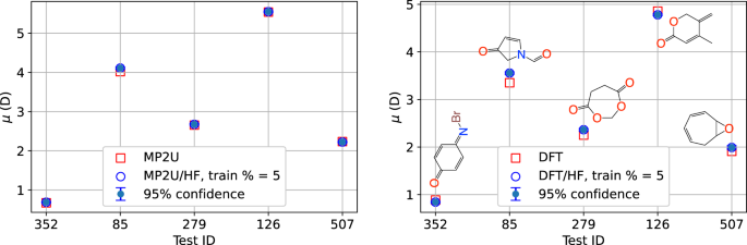
Predictions of the dipole moment μ on the Quinone data set for 5 randomly selected test points: 4-bromoiminocyclohexa-2,5-dien-1-one C₆H₄BrNO (352); 3-oxo-2H-pyrrole-1-carbaldehyde C₅H₅NO₂ (85); 1,3-dioxepane-4,7-dione C₅H₆O₄ (279); 4-methyl-5-methylidenepyran-2-one C₇H₈O₂ (126); 8-oxabicyclo[5.1.0]octa-2,4-diene C₇H₈O (507).

Full size image

QM7bE data set

The RMSE values relating to predictions of E_eff in the QM7bE data set are shown in Fig. 6. As with the Quinone and QM7b data sets, we observe that MFGP-GEM provides the most consistent and accurate results; here PCA-MACCS with 50 principal components was used as the additional descriptor. Corresponding scatterplots are shown Fig. 7. In Supplementary Figs. 9 and 10 we show the equivalent RMSE values and corresponding scatterplots for the STO-3G basis, while comparisons to other methods are shown in Supplementary Fig. 11.

RMSE values pertaining to the prediction of E_eff in the QM7bE data set, with the combinations of lo-fi:hi-fi data and the basis set indicated.

Full size image

Scatterplots of the true vs. predicted E_eff using MFGP-GEM on the QM7bE data set, with different combinations of lo-fi:hi-fi data and different basis sets.

Full size image

The results with MFGP-GEM are highly accurate for all bases, especially for the 6-31G basis, with a minimum R² of 0.94 across all combinations of lo-fi:hi-fi data, basis set and training point number. The map from MP2 to CCSD(T) is the most accurate, with a minimum R² of 0.985. What is particularly noticeable from Fig. 6 and Supplementary Fig. 9 is that only between 16 to 128 lo-fi and hi-fi data points are required for such accuracies, e.g., to reach MAEs of 1.29 kcal/mol and 1.48 kcal/mol (within chemical accuracy) for CCSD(T):MP2(cc-pVDZ) and CCSD(T):MP2(6-31G) requires only 16:16 and 32:32 training points, respectively. For CCSD(T):HF(cc-pVDZ) and CCSD(T):HF(6-31G), MAE values of 2.3 kcal/mol and 2.23 kcal/mol were obtained using 64:64 and 32:32 training points, respectively.

ML-MEGNET and CQML again failed to provide reasonable accuracies using 1:1 low-fi:hi-fi training point ratios. Instead, we used the values from the original papers at 2:1 and 4:1 ratios⁵⁴. Report an MAE value of ~1 kcal/mol with 1024:2048 or 512:2048 training points using ratios of 1:2 or 1:4 for CCSD(T):MP2(cc-pVDZ), respectively. For CCSD(T):HF(cc-pVDZ), the same level of accuracy required 512:2048 or 128:2048 training points⁵⁵. Found that 1024:2048 or 512:2048 CCSD(T):MP2(6-31G) training points were required to reach this level of accuracy. For the larger fidelity gap CCSD(T):HF(6-31G), their method required 1024:4096 or 512:8192 points.

Bandgap and Alexandria data sets

The MAE values on the Bandgap data set are shown in Fig. 8. (ref. ⁵⁴ did not provide RMSE values in their work). Δ-ML and CQML were not implemented since there is no obvious way to generate a suitable descriptor for these methods using the available data. As far as we are aware, MF-MEGNET attains the lowest error on the Bandgap data set in the literature. Fidelities for the Bandgap data are defined by the functional, namely GLLB-SC or HSE for hi-fi and PBE0 for lo-fi. MFGP-GEM is far superior in both cases, especially considering that the best case in Fig. 8 for MF-MEGNET requires 41k PBE0 (lo-fi) points. For HSE:PBE0, MFGP-GEM attains an MAE of 0.18 eV at 512:512 points, and the lowest value attained by MF-MEGNET is 0.36 eV at 41k:4800 points. The comparison for GLLB-SC:PBE0 is similar.

The results are shown for two cases: with GLLB-SC as the hi-fi and with HSE as the hi-fi, using DFT-PBE0 as the lo-fi in both cases. The number of hi-fi points is varied along the horizontal axis. MF-MEGNET-1 and MF-MEGNET-2 refer to 5000 and 41,000 lo-fi PBE0 data points used for training, respectively. For MFGP-GEM the numbers of lo-fi and hi-fi points are equal.

Full size image

Properties such as specific heat capacity rely on the distribution of electronic energy levels and vibrational frequencies, which can be estimated with relatively high accuracy using advanced composite methods. The MFGP-GEM RMSE values on the Alexandria data set are shown in Fig. 9 and Supplementary Fig. 12 for various combinations of lo-fi:hi-fi data, together with results for Δ-ML. MF-MEGNET and CQML again failed. For example, MF-MEGNET (CQML) yielded RMSE values of 103 (1277) J/mol/K and 4.05 (13.1) D for C_V and μ using all of the lo-fi data and 1024 hi-fi points in the case of G2:CBS-QB3. We note that the DFT results used a B3YLP functional and an aug-cc-pVTZ basis, while HF used a 6-311G** basis. ‘Exp’ denotes experimental data in Supplementary Fig. 12. At 64:64 (1024:1024) G4:CBS-QB3 training points, MFGP-GEM yields RMSE and MAE values of 11.8 (8.4) and 8.1 (4.9) kJ/mol/K, the latter of which is 3.2% (1.9%) of the G4 mean absolute value. Supplementary Fig. 13 shows the corresponding scatterplot for only 16:16 training points, for which the R² is 0.997. There are several outliers in the data with values above 1000 kJ/mol/K that are nevertheless extremely well approximated, in particular the value at around 5400 kJ/mol/K. In the case of W1BD:CBS-QB, the accuracy of the (Delta {H}_{f}^{0}) predictions is even higher. The MAE for 64:64 (512:512) training points is 5.2 (3.2) kJ/mol/K, representing 1.8% (1.1%) of the mean absolute value. Supplementary Fig. 13 shows that outliers are again extremely well approximated with only 16:16 points.

RMSE values relating to predictions in selected cases from the Alexandria data set, with the combinations of lo-fi and hi-fi data indicated.

Full size image

The best approximation is achieved for C_V, with all three combinations of hi-fi:lo-fi. In the case of G4:CBS-QB3, the R² is 1.000 and the MAE is 0.45 J/mol/K (0.13% of the mean) at 16:16 training points. Only slightly less accurate are the predictions of S⁰, with MAE values of 0.78, 0.80 and 1.93 J/mol/K at 16:16 training points for W1BD:CBS-QB3, G4:CBS-QB3 and G2:CBS-QB3 (0.27%, 0.23% and 0.58% of the mean absolute value for the respective hi-fi). The results for μ are the least accurate, for the reasons discussed earlier. For DFT:HF and Exp:DFT, the MAEs at 128:128 points are 0.13 and 0.26 D, which are 7.3% and 13.4% of the respective hi-fi mean values. The approximations of α are much more accurate, with equivalent MAE values of 0.30 and 0.24 ų, which are 2.6% and 1.9% of the mean values.

Predictions of C_V and S⁰ and the confidence intervals for 5 randomly selected test points are shown in Fig 10, alongside the experimentally measured values. Equivalent predictions for α and μ are provided in Supplementary Fig. 14. C_V and S⁰ values are influenced by the size of the molecule and the number of degrees of freedom. Popylcyclopentane and methylcyclopentane are aliphatic compounds with flexible acyclic structures. The numerous degrees of freedom associated with rotations and vibrations in aliphatic molecules lead to increased heat capacities and molar entropies. In contrast, aromatic compounds such as 1-fluoro-2-methylbenzene generally have lower C_V and S⁰ values due to the more constrained molecular motion. Naphthalene-1-carbaldehyde has a relatively high polarizability due to the substantial number of π electrons in the highly-conjugated aromatic naphthalene ring. The high polarizability of 1-bromooctane is primarily attributable to the presence of the halogen bromine atom and the long carbon chain. Even with this wide variety of molecules, the predictions are accurate, especially for the thermodynamic properties.

Predictions of C_V and S⁰ from the Alexandria data set for 5 randomly selected test points: 1-fluoro-2-methylbenzene C₇H₇F (165), N-oxonitramide N₂O₃ (509), nitrous acid HNO₂ (731), propylcyclopentane C₈H₁₆ (1885); methylcyclopentane C₆H₁₂ (1699).

Full size image

N − fidelity simulations

Both⁵⁴ and⁵⁵ found that adding more fidelities boosted the accuracy of their multi-fidelity method. We also found this to be the case in most of the examples considered. An illustration of the improvement is provided in Fig. 11, which examines cases with up to 5 fidelities (labeled NFi, N = 2, …, 5). For the definitions of cases 1 and 2 we refer to the caption of Fig. 11. In relation to the QM7bE data, the MAE (R²) reaches 1.12 kcal/mol (0.996) and 1.04 kcal/mol (0.997) for the 6-31G and cc-pVDZ bases, respectively, using 64:64:64 CCSD(T):MP2:HF training points. In the case of STO-3G it reaches 2.21 kcal/mol, which is still very accurate. Scatterplots for the cc-pVDZ and 6-31G cases are shown in Supplementary Fig. 15. The 4Fi models lead to even higher accuracies, with MAEs of 0.99 kcal/mol for both case 1 and case 2 when using 64 points at each fidelity, and 0.91 kcal/mol when using 512 points at each fidelity. The 5Fi models yield even more dramatic improvements, with MAE values of 0.72 kcal/mol in both cases when using 64 points at each fidelity and 0.61 kcal/mol when using 512 points at each fidelity. The dipole moment prediction on the Quinone data set is also significantly improved, with a reduction in the MAE from 0.217 D at DFT:MPR to 0.137 D at HF:DFT:MPR using 20% of the data for training. At 10%, the E₀ RMSE is reduced from 0.33 eV using CCSD:DFT to 0.09 eV using HF:DFT:CCSD. As with adding more training points of the same type, adding further fidelities will eventually lead to diminishing returns.

The quantity and fidelities are indicated in the legends and titles. 4Fi case 1 refers to the fidelities HF-STO-3G, HF-cc-pVDZ, MP2-cc-pVDZ and CCSD(T)-cc-pVDZ. 4Fi case 2 refers to HF-STO-3G, HF-6-31G, MP2-6-31G and CCSD(T)-cc-pVDZ. 5Fi case 1 refers to HF-cc-pVDZ, MP2-6-31G. MP2-cc-pVDZ, CCSD(T)-6-31G and CCSD(T)-cc-pVDZ. 5Fi case 2 refers to HF-STO-3G, HF-cc-pVDZ, MP2-STO-3G. MP2-cc-pVDZ and CCSD(T)-cc-pVDZ.

Full size image

High-fidelity QM simulation methods are generally not suitable for the rapid screening or design of materials. At the very least, such applications would require massive computational resources and budgets. Even when such resources are available, the simulation times could easily be prohibitive for complex molecules, large numbers of molecules, and costly hi-fi methods. Direct ML approaches can suffer from the same problem, since they usually require a large volume of (possibly hi-fi) data. MF methods could well provide a solution in such cases, provided that the lo-fi results are cheap to obtain, which is certainly the case with semi-empirical, HF and some DFT approaches.

In this paper, we leveraged the power of spectral embeddings and autoregressive (Markov) approaches to develop a MF method that is capable of accurate predictions using small numbers of both lo-fi and hi-fi data. We examined its performance on a range of data sets to show that it is generalizable across fidelity combinations, types of molecules and types of output. Unsurprisingly, we find that localized properties of molecules such as μ and α can be more difficult to capture than global properties. The results also suggest that the application of MF methods to the predictions of such properties requires a more careful planning of data acquisition, in that the data from different fidelities must exhibit strong correlations. Pairing methods with shared underpinnings, such as HF and post HF, will likely lead to stronger correlations than pairing methods such as GW and DFT. The N − Fidelity results show that adding more fidelities can dramatically improve the results. This does not mean, however, that it is always prudent to add more fidelities. The improved accuracy has to be weighed against the increased computational costs of acquiring the additional data. In cases where data is available at HF and say G4MP2, it may well be worth generating additional data at the DFT level. There may also be cases in which results at intermediate levels of theory can be acquired efficiently, for example in composite methods.

We investigated relatively simple adjacency matrices in this work and it is possible to use more information related to the molecules. Although we do not expect the results to improve dramatically, further accuracy gains are possible. Another route to improved accuracy is transfer learning, which would allow for different ratios of lo-fi and hi-fi training data, and therefore a fuller exploitation of the short simulations times associated with the former.

Gaussian processes based on spectral graph embeddings via diffusion maps

Backgrounds on the ML and MF methods used for comparison are provided in Supplementary Sections 5 and 6, respectively. Implementations of these methods are described in “Implementations of direct machine learning and other multi-fidelity methods”.

A graph ({{mathcal{G}}}) is an ordered pair (V, E), where V is a non-empty set of vertices or nodes, and E is a set of edges, each of which is an unordered pair of distinct vertices from V. In the context of molecules, the vertices v₁, …, v_n ∈ V in ({{mathcal{G}}}) are identified with the n atoms. The atom properties, such as atom type, position and charge are used as node features. A set of edges E = {(v_i, v_j)∣v_i, v_j ∈ V, v_i ≠ v_j} is defined to represent the bonds, indicating whether or not v_i and v_j are connected. In a weighted graph ({{mathcal{G}}}=(V,E,W)), each edge (v_i, v_j) is associated with a weight w_ij ∈ W, which represents the strength of the relationship between the associated vertices. In molecular graphs, weights (or edge features) can be assigned to the edges between atoms, based on bond properties such as the type, strength and length. Molecular graphs are undirected since the order of the vertices in the edges (v_i, v_j) is immaterial. Moreover, they are connected, since there is a path between any two distinct vertices.

Diffusion maps⁶¹ (see Supplementary Section 4.1) define embeddings on graphs using the concept of a diffusion space. The vertices are embedded isometrically in diffusion space by preserving a diffusion distance. Let ({{mathcal{G}}}) be a weighted molecular graph with vertices V = {v₁, v₂, …, v_n} for a molecule m possessing n atoms. An adjacency or connectivity matrix ({{bf{K}}}={[{K}_{ij}]}_{i,j}in {{mathbb{R}}}^{ntimes n}) can be constructed from the weights w_ij, considering the presence of bonds, bond types, bond strengths or other properties (edge features) by using, e.g., thresholding for a particular feature or a weighted average of the features. The adjacency matrix entry K_ij = w_ij defines a metric (distance or similarity measure) d(v_i, v_j) between nodes i and j. A diffusion process on ({{mathcal{G}}}) is obtained from the diffusion matrix P = D⁻¹K, in which D is the degree matrix. The matrix P is a Markov matrix for a random walk on the graph. t-step transition probabilities are obtained from P^t.

The eigenvalues γ_i of P can be ordered such that 1 = γ₁ > ⋯ > γ_n, with corresponding right and left eigenvectors ({{{bf{r}}}}_{i}in {{mathbb{R}}}^{n}) and ({{{bf{l}}}}_{i}in {{mathbb{R}}}^{n}), respectively. The key quantities required for defining the diffusion maps are the row vectors ({{{bf{p}}}}_{j}^{t}={sum }_{i = 1}^{n}{({gamma }_{i})}^{t}{r}_{ji}{{{bf{l}}}}_{i}) of P^t, j = 1, …, n. Here, r_ji is the j-th component of r_i. The vector ({{{bf{p}}}}_{j}^{t}) defines a probability mass function, with the i-th component being the probability of reaching vertex v_i from v_j in t steps. Diffusion maps ({psi }^{t}:Vto {{{mathcal{D}}}}^{(t)}subset {{mathbb{R}}}^{n}) are defined by ({psi }^{t}({v}_{i})={left({({gamma }_{1})}^{t}{r}_{i1},ldots ,{({gamma }_{m})}^{t}{r}_{in}right)}^{T}), mapping to a diffusion space ({{{mathcal{D}}}}^{(t)}), with preservation of a diffusion distance (Supplementary Section 4.1). The decay in the eigenvalues leads to low-dimensional embeddings ({psi }_{r}^{t}({v}_{i}):Vto {{{mathcal{D}}}}_{r}^{(t)}subset {{mathbb{R}}}^{r}) by restricting ψ^t(v_i) to the first r < n (user chosen) components.

Graphs ({{{mathcal{G}}}}_{m}) can be formed for each molecule m to extract the right eigenvectors and eigenvalues, ({{{{{bf{r}}}}_{i,m}}}_{i = 1}^{r}) and ({{{gamma }_{i,m}}}_{i = 1}^{r}), respectively. Since the molecules have different numbers of atoms n, the r_i,m are padded with 0s such that they all lie in ({{mathbb{R}}}^{widehat{n}}), where (widehat{n}) is the number of atoms in the largest molecule. The set of vectors and eigenvalues can then be concatenated to produce a feature vector representing molecule m

in which ⊕ is used to denote a concatenation. A new graph (widehat{{{mathcal{G}}}}=(widehat{V},widehat{E},widehat{W})) is now defined by associating each node ({widehat{v}}_{m}in widehat{V}) with a molecule m, for which we have a feature vector z_m. An adjacency matrix (widehat{{{bf{K}}}}in {{mathbb{R}}}^{Mtimes M}) can be defined using a kernel function k(z_l, z_m), e.g., the following Gaussian kernel

for some shape parameter s (user chosen). This specifies the metric (widehat{d}(cdot ,cdot )) and also the weights ({widehat{w}}_{mn}in widehat{W}) associated with the edges in (widehat{E}). A diffusion map embedding is performed as above to yield right eigenvectors ({widehat{{{bf{r}}}}}_{m}) and eigenvalues ({widehat{gamma }}_{m}), alongside low-dimensional embeddings ({phi }_{q}^{t}({u}_{j}):widehat{V}to {widehat{{{mathcal{D}}}}}_{q}^{(t)}subset {{mathbb{R}}}^{q}) given by

for some q < M. ({widehat{{{mathcal{D}}}}}_{q}^{(t)}) is a diffusion space and ({widehat{r}}_{ji}) is the j-th component of ({widehat{{{bf{r}}}}}_{i}). Optionally, a descriptor or concatenation of descriptors ({{{bf{d}}}}_{m}in {{mathbb{R}}}^{d}) can be combined with x_m, to produce features ({{{bf{x}}}}_{m}mapsto {{{bf{x}}}}_{m}+{{{bf{d}}}}_{m}in {{mathbb{R}}}^{q+d}), which are fed to the multi-step nonlinear autoregressive model described below. The procedure to extract the x_m is illustrated in Fig. 2.

We assume the autoregressive form ({y}^{F}={eta }^{F}({eta }^{fin {{mathcal{F}}}}({{bf{x}}}),{{bf{x}}})+epsilon ({{bf{x}}})), in which ({{mathcal{F}}}subseteq {F-1,ldots ,1}) is a subset of the fidelity indices. (epsilon | sigma sim {{mathcal{GP}}}left(0,{sigma }^{2}delta ({{bf{x}}},{{{bf{x}}}}^{{prime} })right)) is the error (σ² is the noise variance) and (delta ({{bf{x}}},{{{bf{x}}}}^{{prime} })) is the Kronecker delta function. We note that unlike GPNAR, this is a generalized Markov model with (,{mbox{dim}},({{mathcal{F}}})) steps; that is, ({eta }^{F}perp {{eta }^{f}:fnotin {{mathcal{F}}}}| {{eta }^{f}:fin {{mathcal{F}}}}). A GP prior ({eta }^{F}| theta sim {{mathcal{GP}}}left(0,c(cdot ,cdot | theta )right)) with covariance function (cleft([{{bf{x}}},{eta }^{fin {{mathcal{F}}}}({{bf{x}}})],[{{{bf{x}}}}^{{prime} },{eta }^{fin {{mathcal{F}}}}({{{bf{x}}}}^{{prime} })]| theta right)) containing hyperparameters θ is placed over the latent function. The notation ([{eta }^{fin {{mathcal{F}}}}({{bf{x}}}),{{bf{x}}}]) denotes a concatenation of selected fidelities and x. Since the latent function values ({eta }^{f}({{{bf{x}}}}_{m}^{f})) are not known (unless the computations are error free), we approximate these values by the observations y^f and absorb the error resulting in this approximation into a redefined error. We first define a compact notation

The prior then takes the form ({eta }^{F}| theta sim {{mathcal{GP}}}left(0,cleft({{bf{s}}},{{{bf{s}}}}^{{prime} }| theta right)right)) for a model ({y}^{F}={eta }^{F}left({{bf{s}}}right)+epsilon ({{bf{s}}})), in which ({{{bf{s}}}}^{{prime} } = mathop{bigoplus}nolimits_{fin {{mathcal{F}}}}({eta }^{f}({{{bf{x}}}}^{{prime} })+{epsilon }^{f}({{{bf{x}}}}^{{prime} }))oplus {{{bf{x}}}}^{{prime} }) and ϵ(s) is Gaussian white noise with variance σ². The posterior predictive distribution is

in which ({{bf{C}}}(theta )={[c({{{bf{s}}}}_{m},{{{bf{s}}}}_{{m}^{{prime} }}| theta )]}_{m,{m}^{{prime} }}in {{mathbb{R}}}^{Ntimes N}) is the covariance matrix, N is the number of training points, and ({{{bf{s}}}}_{m}{ = bigoplus }_{fin {{mathcal{F}}}}{y}_{m}^{f}oplus {{{bf{x}}}}_{m}^{F}), recalling that X^f ⊆ X^f−1. The predictive mean and variance at a given s are ({m}^{{prime} }({{bf{s}}}| theta )) and ({c}^{{prime} }({{bf{s}}},{{bf{s}}}| theta )), respectively. The hyperparameters are estimated using a maximum log likelihood

Implementation details

MFGP-GEM was implemented in Python 3.8.17 using the GPy package, and used a maximum likelihood to infer the hyperparameter values based on a square (L₂) loss function and a non-stationary sum of Matérn 5/2 automatic relevance determination (ARD), linear ARD and Gaussian noise kernels. We found that this kernel, or a kernel that replaced the Matérn 5/2 ARD component with a squared-exponential ARD (SEARD) kernel worked better than SEARD or Matérn ARD kernels alone, probably due to the fact that MF problems are essentially sequence problems and therefore not stationary. Structures were created with the MolFromSmiles() function from the Chem library in RDkit. From these structures, two types of adjacency matrices K were considered, ‘bond’ and ‘connectivity’. ‘connectivity’ refers to simple binary-valued entries that indicate the presence or absence of a bond. ‘bond’ included both the presence and type of bond, e.g., single (1), double (2) or triple (3), with 0 used for the absence of a bond. More elaborate adjacency matrices K such as entries that are linear combinations of bond type encodings and atomic weights of the species in the edge could also be used.

For the QM7b data set, the bond information for the adjacency matrix was derived from the Coulomb matrices. For the QM7bE and Bandgap data sets we used the connectivity-based adjacency matrix since only xyz data is available. A bond distance threshold was defined to decide connectivity; those atoms separated by a distance below the threshold were considered connected. For the Alexandria data set, the available InChi representations were converted to SMILEs using the Chem.MolFromInchi() and Chem.MolToSmiles() functions in RDkit. The additional descriptors were generated in Python from SMILEs representations using AllChem in RDkit. All fingerprints and the SoB were assumed to have a size of 1024 bits, while MACCS keys have a size of 166 bits. To generate PCA and SPCA representations we used the scikit-learn package. ACSF and SOAP were implemented with the DScribe package. Where available, the atomic coordinates were used to define the centers in both methods. For each data set, the radial cutoff, number of spherical harmonics and number of radial basis functions were varied in SOAP to achieve the best results. It was found that spherical Gaussian type orbitals were superior to a polynomial basis. Similarly, for ACSF, the radial cutoff and symmetry function parameters were varied to obtain the best fits. These local descriptors were transformed into global descriptors using the averaging option. Zero padding was used to create descriptors of a fixed size, determined by the size of the largest molecule.

Generation of the Quinone data set

Initial geometries were generated from SMILEs representations using RDkit. All calculations were performed using the Python package PySCF⁸³ based on optimized geometries using unrestricted HF (UHF). Subsequent HF calculations were performed with a cc-pVDZ basis. The HOMO energy in HF is determined from ({E}_{{{rm{HOMO}}}}^{{{rm{HF}}}}={varepsilon }_{{{rm{occupied}}}}^{{{rm{HF}}}}), and the LUMO from ({E}_{{{rm{LUMO}}}}^{{{rm{HF}}}}={varepsilon }_{{{rm{unoccupied}}}}^{{{rm{HF}}}}). DFT calculations were performed with unrestricted KS using the B3LYP XC functional. HOMO and LUMO indices were identified from the KS orbital energies and occupancies. MP2 and CCSD calculations used the UHF results as reference wavefunctions. Density-Fitted MP2 was used to obtain the unrelaxed and relaxed dipole moments. Full details of the generation of the data set are provided in Supplementary Section 2.1.

Implementations of direct machine learning and other multi-fidelity methods

The direct GP model, MEGNET and the GCN were implemented in Python, while the CNN and MLP models were implemented in Matlab 2023a. The GP model used GPy, with a maximum likelihood for inferring hyperparameters. The mean values were assumed to be zero, and a SEARD kernel with Gaussian noise was employed. All networks used the square error (L₂) loss function and were trained with the Adam optimizer⁸⁴. The GCN, MLP and CNN architectures described below were found to be optimal using initial hand tuning followed by stochastic grid searches. Initial learning rates of 10⁻³ were used in all cases.

The GCN was implemented in PyTorch using the GCNConv function in PyTorch Geometric. The architecture used is summarized in Table 2. The size of the input space ‘in’ differs according to the data set. For the QM7b data set, padded Coulomb matrices were used to create the graph via the nx.Graph() function in NetworkX. Node features for the j − th atom were set equal to the values in the j − th row of the Coulomb matrix, which describe interactions between the j − th atom and the other atoms in the molecule. An edge feature between nodes j and k was defined by the (j, k) − th value of the Coulomb matrix, which represents an interaction strength. The same procedure was used for the Quinone data set, with Coulomb matrices generated from SMILES using our own custom functions based on RDkit. For the QM7bE data set, pymatgen structures were used to generate the Coulomb matrices.

The direct MEGNET model was implemented according to the recommended structure described in Supplementary Section 5.5. We chose r_cutoff = 5 and n = 100 for the cutoff distance in the GaussianDistance function and the number of features, respectively. For the Quinone data set, the MEGNET get_pmg_mol_from_smiles function was used to convert SMILES representations to pymatgen structures in order to use CrystalGraph. For the QM7bE data set, structures were created from available xyz files⁵⁵ using the pymatgen XYZ and Molecule functions, based on the atomic coordinates and species. The QM7b data set provides only Coulomb matrices, from which we were unable to generate structures.

The CNN architecture is summarized in Table 2. The height H and width W correspond to the number of descriptors and lengths of the descriptor sequences, respectively (we may think of the descriptors as vectors in ({{mathbb{R}}}^{d}) or equivalently as sequences with d terms). In the case of full sequences, rather than PCA versions, the MACCS keys were padded with 0’s to be of length 1024 if they were used in combination with other descriptors. The MLP architecture is also shown in Table 2. The input was a descriptor or concatenation of descriptor sequences, resulting in a length ‘in’.

The GP multi-fidelity models were again implemented in Python using GPy. GPNAR and GPLAR followed their original formulations^51,57, employing the SEARD kernel with Gaussian noise. Stochastic collocation was also implemented according to the original formulation⁵⁸. MF-MEGNET was implemented according to the original work⁵⁴ by appending a fidelity index to the structures, namely 1 for low and 2 for high, under the ‘state’ key. These variables are passed as global features to MEGNET.