Research on collaborative scheduling strategies of multi-agent agricultural machinery groups

Introduction
With the continuous improvement of China’s agricultural modernization level, the traditional decentralized scheduling mode for agricultural machinery has become inadequate for current agricultural production needs due to its lack of a global perspective and effective cost control in scheduling costs1. The agricultural machinery industry gradually is increasingly exhibiting a pattern of resource mismatch, characterized by “organic households having no work to do, while non-organic households have work but no machines available”2. Currently, inter-area machine harvesting has emerged as a relatively mature scheduling model, with harvesting operations expanding from wheat to corn and rice, demonstrating significant vitality. In January 2022, the Ministry of Agriculture and Rural Affairs issued the “14th Five-Year Plan” National Agricultural Mechanization Development Plan, which encourages the promotion of intelligent upgrading and transformation of agricultural machinery, and accelerates the popularization and application of intelligent agricultural machinery3. As the number of agricultural machines increases and the process of intelligentization accelerates, a key issue that must be addressed is how to scientifically plan and schedule the operational paths of the harvesters in order to improve agricultural production efficiency, reduce costs, and maximize the utilization of harvester resources.
Currently, traditional heuristic algorithms such as the Genetic Algorithm (GA)4, Simulated Annealing Algorithm (SA)5, and Ant Colony Optimization Algorithm (ACO)6 have been widely employed to address the path planning challenges associated with agricultural machinery operations.Haixiang Guo et al.7 proposed a single dispatch center path problem and used hybrid heuristic algorithm, specifically a hybrid genetic algorithm and a hybrid ant colony algorithm to develop a reasonable and effective path planning scheme.MATEI et al.8 expanded the Vehicle Routing Problem (VRP) by designing and implementing a hybrid heuristic model that integrates a genetic algorithm, a local search mechanism, and a migration policy to solve the single dispatch center path planning issue. Zhou Qian et al.9 introduced a genetic TABU search algorithm that combines TABU search with genetic operators to solve the problem of regional scheduling of vehicles with a single dispatch center.Zhou Xiancheng et al.10 proposed an improved ant colony algorithm targeting the green vehicle path problem across multiple dispatch centers, and with experimental results indicating that the algorithm can effectively plan the distribution path of vehicles while significantly reducing the total logistics and distribution costs.Wei Ming et al.11 developed a model for the collaborative planning of UAV transport routes and trajectories in a multi-order dispatch center for logistics and distribution, optimizing the best UAV transport routes, operational time and trajectory scheme.Chen Yanyi et al.12 proposed an improved ant colony-genetic algorithm for addressing the path planning problem of fresh food distribution across multiple dispatch centers.The experimental results demonstrate that this algorithm is more efficient than traditional algorithms, effectively alleviating the conflict between the timeliness of distribution and the uncertainty of distribution time.MEH et al.13 introduced a variable contraindicated neighborhood search algorithm that incorporates contraindicated moves during the jitter phase of the variable neighborhood search algorithm to tackle the Multi-Depot Vehicle Routing Problem (MDVRP). Gu et al.14 proposed a method to solve the single dispatch center vehicle path problem using an artificial bee colony algorithm.This approach reduces the MDVRP to a single dispatch center problem by clustering the dispatch centers, modifies the artificial bee colony algorithm to generate solutions for each dispatch center, and proposes a co-evolutionary strategy for generating a comprehensive MDVRP solution.Qui Hao et al.15 addressed a three-stage optimization algorithm employing an ant colony algorithm for a multi-dispatch center vehicle path problem, incorporating three-dimensional loading constraints with the aim of minimizing the distance traveled by the vehicles.
With the rapid development of machine learning technology, Deep Reinforcement Learning (DRL)16 has been extensively applied to the path planning problem, offering a novel perspective and solution for addressing the operational path planning challenges faced by multiple harvesters and dispatch centers in complex environments.DRL effectively integrates the robust perceptual capabilities of Deep Learning with the efficient decision-making mechanisms of Reinforcement Learning, demonstrating exceptional performance in managing complex tasks and environments. Ge Bin et al.17 proposed an end-to-end deep reinforcement learning network architecture to address the vehicle path planning problem with a single dispatch center. They designed an edge aggregation graph attention network encoder and a multi-head attention decoder.The experimental results demonstrated the effectiveness and superiority of their framework in solving this type of problem.Similarly, Jiang Ming et al.18 introduced an end-to-end deep reinforcement learning method based on a multi-pointer Transformer.This model showcases its superiority by enhancing both the encoder and decoder.When compared to existing heuristic algorithms and other deep learning methods, their algorithm maintains a rapid solving capability within a small optimal gap, effectively addressing the vehicle path problem for a single dispatch center. Huang Yan et al.19 applied deep reinforcement learning algorithms to a vehicle path planning scenario at a single dispatch center, aiming to identify the shortest path by leveraging the rewards obtained from the interaction of intelligent agents with the environment, thereby addressing the vehicle path problem in an end-to-end manner. Chen et al.20 proposed a deep reinforcement learning based encoder-decoder framework for tackling the hybrid delivery and pickup vehicle routing problem within a single dispatch center. This framework employs a Graph Neural Network (GNN) as the encoder structure to extract instance features, while a decoder with an attention mechanism translates the detailed routes into sequences, ultimately yielding high-quality solution. Arishi et al.21 introduced an algorithm based on a novel multi-intelligence deep reinforcement model to solve the multi-dispatch center problem. They evaluated the performance of this approach through extensive experiments, demonstrating that the model could generate high-quality solutions in real-world environments. Lei Kun et al.22 prensented an end-to-end deep reinforcement learning framework designed to enhance the efficiency of solving the vehicle path problem involving multiple dispatch centers. This framework utilizes a Transformer-based decoder combined with an attention mechanism, and its feasibility and effectiveness were verified using both randomly generated arithmetic cases and publicly available standard arithmetic cases. Li et al.23 employed a multi-head attention (MHA)24 mechanism within a multi-dispatch center scenario to integrate various types of embeddings from both the network and the environmental state at each step.This approach facilitated the accurate selection of the next accessed node and the construction of the path. Additionally, they introduced a dispatch center rotation enhancement method to optimize the decoding process. Wang Wanliang et al.25 developed a policy network comprising multiple intelligences that utilized both single-head attention (SHA) and multi-head attention mechanisms.They implemented a policy gradient algorithm to derive an efficient solution. while incorporating the 2-opt26 local search technique alongside a sampling search technique to optimize the multi-dispatch center vehicle path problem. Yu et al.27 proposed an enhancement to improve the pointer network by simplifying the encoder based on recurrent neural networks, thereby offering a more efficient solution to the vehicle path planning challenge in multiple dispatch centers.
In summary, while deep reinforcement learning algorithms demonstrate strong performance in addressing path planning issues, there is a notable gap in research concerning the multi-harvester path planning problem involving multiple scheduling centers within the agricultural sector.Therefore, this paper aims to investigate a collaborative job scheduling scheme for multi-machines across multiple scheduling centers., utilizing a deep reinforcement learning approach. This will be achieved by developing an encoder-decoder architectural model integrated with a multi-head attention mechanism, analyzing various types of data from the farmland, and designing an enhanced REINFORCE algorithm25 for model training.
Problem and model
Problem description
This section describes the problem of multiple harvester path planning involving multiple dispatch centers. Specifically, there are n harvester dispatch centers located within a defined region, each of which has k harvesters to provide operation services for m pieces of farmland distributed in different locations.The dispatch center must take into account several factors, including the performance of the harvester, the geographic locations of the farmland, the size of the farmland plots, and other relevant considerations, in order to effectively plan the operation path for the harvester.The objective is to ensure that all farmland is cultivated while minimizing scheduling costs.The following assumptions are made to facilitate the study of multi-dispatch center job path planning.
-
(1)
Each harvester has the uniform performance and travels at a constant speed.
-
(2)
The number of harvesters assigned to each dispatch center does not exceed its capacity limit.
-
(3)
Each harvester departs from the dispatch center and returns upon completing its operation.
-
(4)
The effective operating hours of the harvester must not exceed the maximum allowable effective operating hours.
A schematic diagram illustrating the multi-harvester path planning problem with multiple dispatch centers is presented in Fig. 1.

Schematic diagram of the multi-harvester path planning problem with multiple dispatch centers.
Mathematical model for the multi-dispatch-center multi-harvester path planning problem
To formulate the multi-harvester path planning problem with multiple dispatch centers, the relevant variables are defined in this section as follows.
The dispatch center collection is (Ac={{h}_{1},{h}_{2},…,{h}_{i}},i epsilon [1,n]),The collection of farm work sites is (:X={{x}_{n+1},{x}_{n+2},…,{x}_{j}},jepsilon[n+1,n+m]),The harvester dispatch center and farm operation points are merged into a collection of dispatch nodes denoted as (:Y={{s}_{e},{d}_{e}},{s}_{e}={{u}_{e},{v}_{e}},eepsilon[1,n+m]).(:{s}_{e}) denotes the coordinates of the scheduling node, and (:{d}_{e}) denotes the operation time required for the harvester to complete the job task of scheduling node e.The total harvester fleet collection is (:COHC={{hc}_{11},{hc}_{12},…,{hc}_{ir}}), (:iepsilon[1,n],repsilon[1,k]), (:{hc}_{ir}) denotes the r-th harvester in the i-th dispatch center.The collection of effective operating hours of the harvester fleet is (:U={{u}_{11},{u}_{12},…,{u}_{ir}}.iepsilon[1,n].repsilon[1,k]),(:{u}_{ir}) denotes the effective length of time required for the r-th harvester at the i-th dispatch center to complete the operation task.The main parameters are defined as shown in Table 1.
The mathematical model for the multi-harvester path planning problem, involving multiple dispatch centers is developed with the objective of minimizing scheduling costs.The objective function is defined as follows.
The constraints are as follows.
Equation (1) represents the minimum dispatch cost as an objective function, which is solely dependent on the transfer distance between harvester plots, and (:{D}_{opr}:text{t}text{a}text{k}text{e}text{s}:text{t}text{h}text{e}:text{v}text{a}text{l}text{u}text{e}:1:text{w}text{h}text{e}text{n}:text{t}text{h}text{e}:text{t}text{a}text{s}text{k}:text{a}text{t}:text{a}text{s}text{s}text{i}text{g}text{n}text{m}text{e}text{n}text{t}:text{p}text{o}text{i}text{n}text{t}:p:text{i}text{s}:text{c}text{o}text{m}text{p}text{l}text{e}text{t}text{e}text{d},:text{a}text{n}text{d}:0:text{o}text{t}text{h}text{e}text{r}text{w}text{i}text{s}text{e}), Eq. (2) indicates that each harvester commences its operation from the dispatch center and returns to the dispatch center upon task completion, Eq. (3) indicates that only one harvester is permitted to operate on each farmland plot. Equation (4) indicates that the actual operating hours of each harvester must not exceed the maximum effective operating hours.
Algorithm description
This section addresses the multi-harvester path planning problem with multiple dispatch centers through the following steps. (1) modeling the problem as a Markov Decision Process (MDP)19 and constructing a deep reinforcement learning environment. (2) developing a decision network based on the self-attention mechanism which utilizes the current state of the harvester to select the next operational farmland through a hybrid action selection strategy. (3) employing a reinforcement learning strategy gradient algorithm to train the network, thereby fully capturing scheduling process and deriving the optimal scheduling strategy for multiple scheduling centers. (4) applying a 2-opt local search strategy to refine the scheduling scheme output from the model, enhancing the overall the path quality. The solution flowchart for the multi-scheduling center multi-harvester path planning problem is illustrated in Fig. 2.

Flowchart for solving the multi-harvester path planning problem with multiple dispatch centers.
Build an intensive learning environment with multiple dispatch centers and multiple harvesters
The multi-harvester path planning problem, involving multiple dispatch centers, is framed as a sequential decision-making challenge. In this process, each harvester departs from its respective dispatch center, executes the designated operational task, and records the distance between the departure point and the current farmland location, Upon completion of .the current farmland task, the scheduling center dynamically adjusts its strategy based on the harvester’s current state and intelligently determines the next farmland location to be addressed.This iterative process continues until all fields have been fully operationalized, with the objective of minimizing overall operational costs, as well as reducing unnecessary travel distances and resource consumption.
The multi-harvester path planning problem with multiple dispatch centers can be framed as a Markov Decision Process(MDP).Addressing this issue requires the construction of a reinforcement learning environment grounded in MDP framework.The environment comprises a state space S, an action space A and a reward function R.
State Space: The state is defined as (:S={{ob}_{ire}^{t},{m}_{ir}^{t}},eepsilon[1,n+m]),where (:{ob}_{ire}^{t}) represents the position information of the r-th harvester from dispatch center i at farm operation point e at time t, as well as the duration required to complete the current farm operation task.(:{u}_{ir}^{t}) represents the remaining effective operation time of the r-th harvester in dispatch center i after time t.
The action space is defined as the set of dispatch nodes at which a harvester can choose to perform a job task at moment t,(:{A}^{t}=left{{A}_{ire}^{t}:right},eepsilon[1,n+m].) Specifically, (:{A}_{ire}^{t}) represents the action of the r-th harvester, originating from the i-th dispatch center moving to the e-th dispatch node to perform a task at time t.
In reinforcement learning, the reward function is regarded as a evaluation criterion for agent’s behavior.In this paper, the reward function is defined as the negative of the total transfer distance of all harvesters, i.e.
Constructing deep learning neural network models
In this paper, an encoder-decoder architecture is employed to address the multi-harvester path planning problem involving multiple scheduling centers.The encoder is tasked with embedding the set of scheduling nodes and effectively mapping them into a feature encoding that captures the relationships among scheduling centers and operational points on the farm.The decoder, in turn, selects the optimal operating farm for each harvester in the current state, utilizing the feature codes generated by the encoder alongside operational information during the scheduling process, which includes data from other scheduling centers, the status of the farm’s operational points, and the remaining effective operating hours of the harvester. The encoder-decoder model is illustrated in Fig. 3.
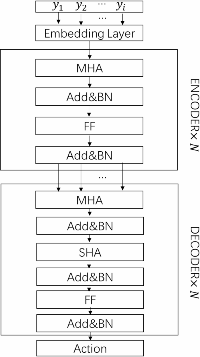
Encoder-decoder model. Note: Add&BN denotes Residual Connections and Batch Normalization; FF denotes feed forward layer.
Designing the encoder
The encoder converts the set of scheduling nodes into feature vectors.In this section, the encoder is composed of an embedding layer and three independent self-attentive components, all sharing the same structure.Each self-attention component comprises of a multi-head attention layer and a feed forward (FF) layer24. To enhance network convergence, stability and generalization.Residual Connections and Batch Normalization are incorporated into both MHA and FF layers.
The encoder processes the set of scheduling nodes by utilizing the embedding layer and the self-attentive component to produce high-dimensional feature representations that incorporate contextual information from the graph node features.Initially, the embedding layer applies a linear transformation to the input scheduling node set (:{Y}_{e}), generating an initial feature vector ({h}_{e}^{left(0right)}) for the scheduling node set,(:eepsilon[1,n+m]), i.e.
where (:W) and (:b) denote the network parameters of the encoder embedding layer and the initial feature vector dimension is (:{d}_{h}=128).
The feature vector (:{h}_{e}^{left(0right)}) output from the embedding layer serves as the initial input to the self-attention component, where the multi-head attention mechanism is employed to extract feature information from the initial feature vector across various dimensions.(:{h}_{e}^{left(0right)}) is first mapped to a query vector (:{Q}_{z}), key vector (:{K}_{z}), and value vector (:{V}_{Z}) used by the encoder through a linear mapping,(:zin:[1,H]), z denotes the different heads of attention and H represents the total number of heads in the multi-head attention, H = 8, i.e.
where (:{W}^{x}) denotes the network parameters. Perform a dotwise multiplication of (:{Q}_{z}) and (:{K}_{z}) in each attention head, scaling the result by (:sqrt{{d}_{k}}) dimensions, where (:{d}_{k}) represents the dimension of the k-vector.The outcomes of this operation are then normalized and dot-multiplied with (:{V}_{z}) using the softmax function to derive the attention vectors (:{L}_{z}) for the various attention heads.
The attention vectors of the various attention heads are merged to obtain the final attention matrix L.
The attention matrix L is updated after the feed-forward layer into a feature vector (:{h}_{e}^{left(1right)}) that can further represent the relationship between the set of scheduling nodes, These feature vectors are continuously updated to new feature vectors (:{h}_{e}^{left(lright)}) by subsequent encoders,(:lepsilon[1,N]), The average value of (h_{text{e}}^{left(text{l}right)}) is taken as the graph node feature (:h_{text{g}text{r}text{a}text{p}h}) that represents the contextual information.
Designing the decoder
The decoder calculates the probability of scheduling the set of nodes based on the output of the encoder. In this section, the decoder comprises an embedding layer, a multi-head attention layer and a single-head attention layer.The input to the decoder consists of two components. the output of the encoder and the set of scheduling nodes The output of the encoder, in turn, includes node embeddings (:{h}_{e}^{left(lright)})and graph node features (:{h}_{graph}).
The embedding layer of the decoder integrates the feature vector (:{h}_{e}) associated with the set of scheduling nodes that have completed the job, along with the remaining effective job duration (:{u}_{t}) of the harvester, to serve as the contextual information (:{s}_{cnt}left(tright)) for the current state.
where (:{W}^{{c}_{1}}) and (:{b}^{{c}_{1}}) are the network parameters of the decoder embedding layer.The feature vector (:{h}_{e}) is derived through a linear mapping to the key vector (:{K}_{fixed}) and the value vector (:{V}_{fixed}) of the decoder.The query vector (:{Q}_{fixed}) of the decoder is formulated by splicing the graph node features (:{h}_{graph}) with the current context information (:{s}_{cnt}left(tright)) following a linear mapping.The attention score (:{G}_{z}) for each SHA is calculated from the query vector in conjunction with the dot product of the key vectors.The calculation process adheres to specific rules to exclude scheduling nodes that are not operable by the harvester. (1) farmland points that have already been processed by the harvester. and (2) farmland points where the time required to complete the farmland operation task exceeds the harvester’s remaining effective operation time .
where (:{G}_{z}) denotes the attention scores for different attention heads.
The attention vectors for different attention heads are denoted as.
The final attention matrix M is denoted as.
The attention matrix M is mapped to the query vector (:{Q}_{sha}) of the single-head attention mechanism in the single-head attention component through the linear layer, and the final attention score is computed through the single-head attention mechanism and the result is scaled to (:[-C,C]) using the tanh function.
Next, the probability distribution (:{p}_{i,e}) for choosing different sets of scheduling nodes is obtained by normalizing the process using the softmax function. i.e.
Based on the previously obtained probability distribution (:{p}_{i,e}), the set of scheduling nodes where the harvester is required to operate can be identified in accordance with the action selection policy.
Optimizing strategy networks for training
This section employs the REINFORCE algorithm with a rollback benchmark, an enhanced policy gradient algorithm for reinforcement learning that mitigates the variance of policy gradient estimation and enhances training stability.Initially, the cumulative returns from the execution of strategies by individual harvesters are computed, and these returns are subsequently utilized to calculate the strategy gradient, which is then used to update the parameter (:theta:) of the harvester’s strategy network parameter.
For a given farmland state s, the policy network (:{pi:}_{theta:}) outputs a vector (:{p}_{theta:}left({pi:}_{t}right|s)) of action probabilities for each harvester based on this state, which is selected by sampling to form a joint policy (:{pi:}_{t}=sampleleft[{p}_{theta:}right(pi:left|sright)]); The benchmark network (:{pi:}_{bl}) then outputs the joint policy (:{pi:}_{t,bl}=greedyleft[{p}_{{theta:}^{bl}}right(pi:left|sright)]) in a greedy selection manner based on the action probability vector (:{p}_{{theta:}^{bl}}left({pi:}_{t}right|s)) output by the benchmark network.Monte Carlo method is used to evaluate the expected cumulative return of the strategy (:Jleft(theta:right|s)={E}_{{p}_{theta:}left(sright)}[text{G}left({uppi:}right)]),where (:Gleft(pi:right)) is the cumulative return of the strategy (:pi:). The REINFORCE algorithm with benchmark is utilized to calculate the strategy gradient with the following formula:
Subsequently, the parameters of the policy network are updated utilizing the Adam optimization algorithm, which is a gradient descent-based method.
The benchmark network is utilized to evaluate the current state of the farm, denoted as s,and to determine difficulty of the task. This assessment allows the policy network to adjust and optimize its behavior more effectively. The(::{pi:}_{bl}) is updated and compared to the (:{pi:}_{theta:}) during the training process.If the output of the strategy network significantly surpasses that of the benchmark network and passes a t-test at a significance level of (:{alpha:}^{prime})(set to 0.05), a rollback update of the benchmark network, i.e.,(:{theta:}^{bl}to:theta:), is executed. This process facilitates the learning and enhancement of the overall strategy network.The specific training process is illustrated in Fig. 4.
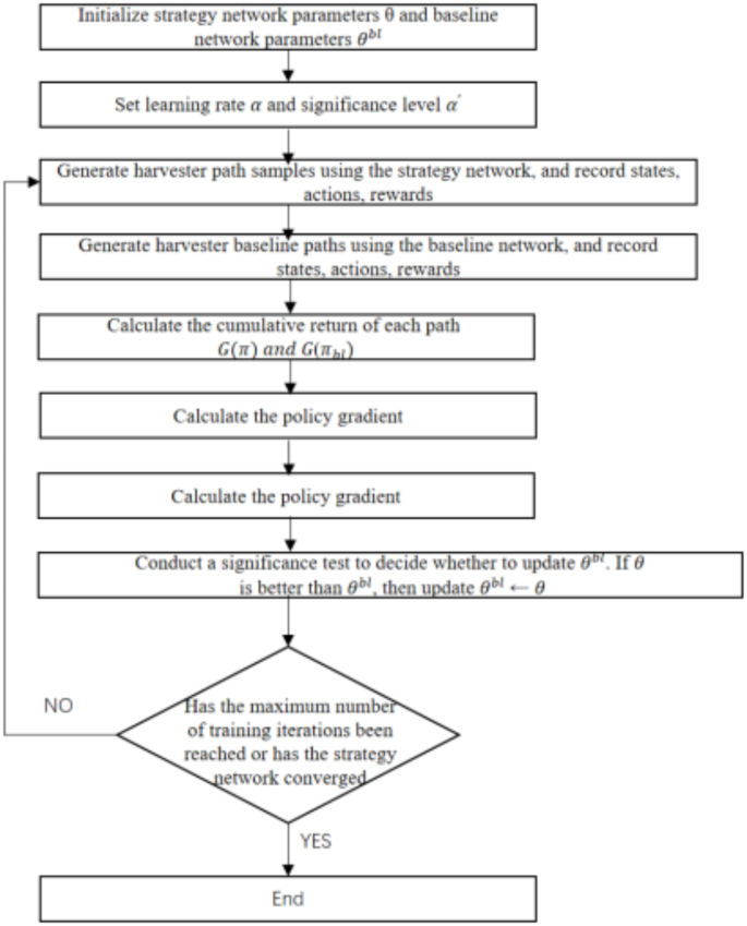
Training flow chart.
Action selection strategy
During the training process for multi-harvester path planning across multiple dispatch centers, the benchmark network (:{pi:}_{bl}) and the policy network (:{pi:}_{theta:}) employ distince action selection strategies.The former utilizes a greedy action selection strategy, while the latter adopts a random sampling action selection strategy.In the case of the benchmark network, the greedy action selection strategy consistently selects the action with the highest expected return at each decision step, thereby ensuring the stability and efficiency of path planning.Conversely, the policy network implements a random sampling action selection strategy, which randomly selects actions based on the action probability distribution, rather than being confined to the action with the highest probability.This approach enhances decision diversity and enables the policy network to explore a broader range of potential paths, ultimately facilitating path optimization.
In this problem, the benchmark network and the strategy network serve distinct roles. The benchmark network is utilized to evaluate the complexity of the problem, employing a greedy action selection strategy to swiftly obtain effective evaluation metrics.Specifically, the benchmark network consistently selects the action with the highest expected return in each state, thereby providing a reliable criterion for path planning. Conversely, the strategy network adopts a randomized action selection strategy to enhance its evaluation of decision-making capabilities in path planning.By randomly sampling from the action probability distribution, the strategy network can explore a broader range of potential paths, avoid local optima, continuously refine the path selection strategy, and ultimately enhance the overall planning effectiveness.
Local search strategy
To address the issue of increased path length due to crossings during harvester operation, a 2-opt local search strategy is introduced in this section.
This strategy minimizes path crossings by exchanging two edges within the path, thereby effectively reducing the distance traveled by the harvester. The strategy iteratively refines the path until it either reaches a local optimal solution or meets a predefined stopping condition. The specific operational steps are as follows.
-
(1)
Iterate over each path operated by the harvester.
-
(2)
Two edges of the current job path are randomly selected and swapped.Specifically, the two edges are removed and the remaining ends are reconnected to form a new job path.
-
(3)
If the length of the new path is shorter than that of the current path, update the current path, reset the number of iterations to 0, and return 1.Otherwise, increase the number of iterations and return 1.
-
(4)
If the maximum number of iterations is reached and the path has not improved, the 2-opt local search concludes, and the current path is returned as the optimal path.
Test results and analysis
Training data
According to the formulation of Eq. (5) in Section 2.1, the reward value is defined as the negative total transfer distance of all harvesters. This value influences the advantages and disadvantages associated with the harvester’s choice of action strategy. Consequently, as the number of training steps increases, the reward value progressively approaches an optimal state and attains a smooth equilibrium.
In the initial stage of model training, the understanding of environmental changes is insufficient, resulting in a low initial reward value that gradually increases. By the time the number of training steps reaches 150,000, the reward value begins to stabilize, indicating that the model is adapting to in the environmental changes. At 200, 000 training steps, the model demonstrates a capacity to quickly adapt to these changes and effectively plan the optimal path with the lowest scheduling cost. The trend of the reward value is illustrated in Fig. 5.
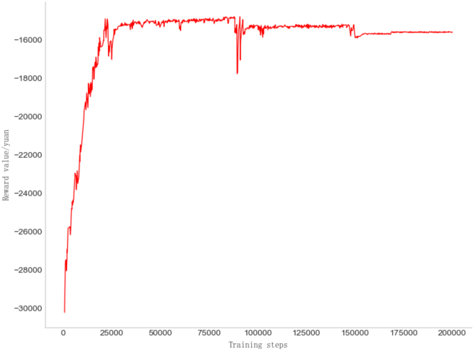
Schematic representation of the variation of reward values with the number of iterations.
Experimental data
In this section, three agricultural machinery dispatch centers, each serving 50 farmlands, were randomly selected for experiments based on the spatial distribution data (36°–41° N, 113°–117° E) of maize cultivation in Hebei Province obtained from remote sensing images.The harvester model utilized is Ward’s semi-fed 4LB-150AA grain combine harvester, which has a fuel consumption rate of approximately 1.7 L/km.The average diesel fuel price from April to July 2024 was around 8.2 Yuan/L, resulting in the harvester’s transfer cost per kilometer being set at 14 Yuan.Due to heavy workload and time constraints during the busy farming season, the harvester often operates continuously.Considering this practical scenario, the effective operation length of the harvester is established at 24 h. To evaluate the advantages of the MCMPP-DRL algorithm proposed in this paper for the multi-dispatch center harvester path planning problem, a comparison is made between the MCMPP-DRL algorithm and other approaches, including the genetic algorithm, simulated annealing algorithm and ant colony optimization algorithm. The information regarding the selected farmland operating points is presented in Table 2.
The farmland operation point serial numbers 0, 1, and 2 correspond to the three dispatch centers, resulting in an operation area of 0 hectares. The remaining information pertains to the farmland operation point.
Results
For simplicity, the scheduling cost results for the three scheduling centers, which include 20, 40, 50, 70, 100 and 120 pieces farmland are abbreviated as (:{MC}_{3-20}), (:{MC}_{3-40}), (:{MC}_{3-50}), (:{MC}_{3-70}), (:{MC}_{3-100}) and (:{MC}_{3-120}). The scheduling cost results for the four algorithms are presented in Table 3.
As can be seen from Table 3, the harvester operating paths of the MCMPP-DRL algorithm proposed in this paper are better than the optimal paths generated using the GA, SA, and ACO algorithms, and therefore achieve the lowest scheduling cost.
Discussion
In order to exclude special experimental data and to further verify the applicability of the algorithm, farmlands of different sizes were selected for comparative analysis in the corn-growing area of Hebei Province. For the three dispatch centers, 20 farmlands, 40 farmlands, 50 farmlands, 70 farmlands, 100 farmlands, and 120 farmlands were selected for the experiment, and five different groups of farm operation sites were selected based on six different sizes of farmlands. Each algorithm was run 10 times and the set of results with the best performance in each experiment was taken out to compare the cost of harvester scheduling under different farmland sizes. The experimental results are presented in Table 4.
As demonstrated in Table 4, the MCMPP-DRL algorithm outperforms the heuristic algorithm iregarding solution quality for problems of sizes MC3–20, MC3–40, MC3–50, MC3–70, MC3–100 and MC3–120. Consequently, the MCMPP-DRL algorithm results in a reduction in harvester costs. Table 5 illustrates the performance improvement in harvester scheduling costs when using the MCMPP-DRL algorithm compared to the heuristic algorithm.
As illustrated in Table 5, the optimization of the MCMPP-DRL algorithm regarding scheduling costs varies in effectiveness across different problem sizes when compared to the heuristic algorithm.this suggests that the MCMPP-DRL algorithm can yield superior experimental results.
As illustrated in Table 6, the disparity between the average costs of each algorithm and the MCMPP-DRL algorithm becomes increasingly pronounced as the number of farmlands increases, while the number of scheduling centers remains constant. This observation further substantiates the effectiveness and rationality of the MCMPP-DRL algorithm. Additionally, Table 7 presents the performance improvement in the average scheduling cost of harvesters when calculated using the MCMPP-DRL algorithm in comparison to the heuristic algorithm.
Tables 6 and 7 further analyze the performance optimization of the MCMPP-DRL algorithm in comparison to the heuristic algorithms, specifically as the number of farmlands varies in the context of three scheduling centers. To more intuitively illustrate the advantages of the algorithm presented in this paper, the average performance of scheduling cost of the MCMPP-DRL algorithm alongside the three heuristic algorithms across different numbers of farmlands is compared and analyzed. The results of this comparison are depicted in Fig. 6 through 11.

Comparison of average cost of different algorithms for 20 farmlands.
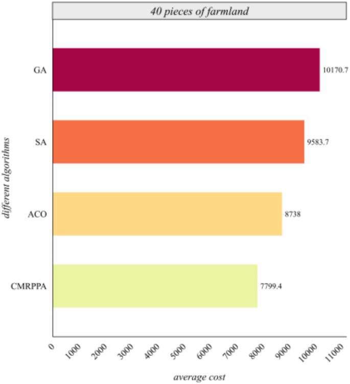
Comparison of average cost of different algorithms for 40 farmlands.
Figure 6 shows that the scheduling cost of the MCMPP-DRL algorithm is significantly lower than that of the other three heuristic algorithms, demonstrating the advantages in scheduling small-scale farmland. Figure 7 shows that as the number of farmland increases, the MCMPP-DRL algorithm still maintains a low scheduling cost, while the cost of the other heuristics increases, reflecting the stability of the MCMPP-DRL algorithm. Figure 8 shows that the advantage of MCMPP-DRL algorithm is more obvious at medium-sized number of farmlands, and the scheduling cost is significantly lower than other algorithms. Figure 9 shows that the MCMPP-DRL algorithm continues to exhibit lower costs, while the heuristic algorithm has a more pronounced trend of increasing costs. Figure 10 demonstrates that the MCMPP-DRL algorithm continues to excel in cost control in large-scale farm scheduling problems, well below the other algorithms. Figure 11 shows that the MCMPP-DRL algorithm maintains the lowest scheduling cost even with a larger number of farmlands, demonstrating superiority and applicability in complex scenarios.

Comparison of average cost of different algorithms for 50 farmlands.

Comparison of average cost of different algorithms for 70 farmlands.
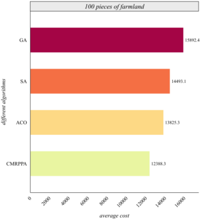
Comparison of average cost of different algorithms for 100 farmlands.

Comparison of average cost of different algorithms for 120 farmlands.
In summary, the MCMPP-DRL algorithm always provides a more economical scheduling solution, regardless of the variation in the number of farmlands.
Conclusion
To effectively reduce the scheduling cost of harvesters, a new algorithm MCMPP-DRL based on deep reinforcement learning is proposed.Different scheduling centers with varying numbers of farmlands in the corn planting area of Hebei Province were randomly selected for simulation experiments. The performance of the MCMPP-DRL algorithm was compared with that of genetic algorithms, simulated annealing algorithm and ant colony optimization algorithm, demonstrating significant advantages in cost reduction.The experimental indicate that the scheduling cost of the MCMPP-DRL algorithm decreases by at least 9.66% compared to the ant colony optimization algorithm, 14.34% compared to the simulated annealing algorithm, and 24.41% compared to the genetic algorithm across various problem sizes.This further substantiates the effectiveness of the proposed algorithm in minimizing scheduling costs. Additionally, this paper analyzes various influencing factors in actual harvester scheduling scenarios, such as fuel consumption and diesel prices and sets these parameters reasonably to ensure that the experimental results possess practical reference value and application prospects.
The research in this paper has the following limitations: first, due to the complexity of the scheduling scenarios, the effectiveness of the proposed method is only initially verified by small-scale practical scenarios, and experimental testing and verification of large-scale practical scenarios need to be further carried out in future work; second, this paper only investigates the co-scheduling problem of the same type of harvester, and does not involve the co-scheduling optimization of a wide range of heterogeneous harvesters. Therefore, the future research direction will focus on the validation of large-scale actual scenarios and the optimization of the cooperative scheduling of heterogeneous agricultural machines to improve the overall efficiency under complex operation scenarios.

Responses