Sensitivity of mesoscale modeling to urban morphological feature inputs and implications for characterizing urban sustainability
Introduction
Urban heat is one of the world’s most significant climate killers1, and it is extremely inequitable – harming the poor, elderly, and otherwise overburdened [e.g.,2,3]. Deaths from urban heat are rising4, and with each new heatwave, the consequences of within-city heterogeneity in urban heat exposure, both indoor and outdoor, become more apparent. Understanding how built environments amplify or mitigate extreme heat within specific neighborhoods is critical to improving urban resilience to future heat extremes5,6. Urbanization and urban growth are defining characteristics of this century, with as much urban infrastructure to be built as currently exists7,8. Understanding the connections between urban form and outdoor heat exposure can support heat mitigation within existing cities and the design of future urban environments. However, characterizing urban heat at sufficiently high resolution to assess the impact of variations in the built environment is a substantial scientific challenge. We know that urban heat can vary spatially by as much as 4–6 °C (7-11 °F) across an urban neighborhood9,10, with large and localized effects on safety and habitability. Heterogeneity in urban heat, especially under future climate conditions, is best assessed through high-resolution numerical weather models. However, while much successful work in representing urban parameters within these models has been accomplished, the extent to which these models are responsive to variations in the resolution of the representation of urban form within them is poorly understood. In order to discern both the effect of morphological inputs on urban heat characterization and the importance of that variance for assessing the equity implications of current and future heat exposure, we assess the influence of four different representations of urban form in numerical weather simulations on urban heat profiles and the implications of their results regarding the assessment of inequality in urban heat exposure to overburdened communities.
It has long been known11 that the variety of surface roughness elements, including buildings in an urban area as numerical weather model parameters, contributes thermal effects to the system in the form of increased absorption of solar radiation, reduction of turbulent sensible heat transfer out of the system, and reduction of long-wave radiation loss from neighborhoods due to multiple building energy reflection and combined neighborhood building shielding. Recently, statistical analysis performed by12 showed that intraurban spatial variability of local diurnal temperature range is positively associated with mortality in neighborhoods that are exposed to larger temperature changes and include lower income populations. Propitiously, the introduction of more granular distinctions in land use and land cover within physical models has opened research avenues for including the communication of a neighborhood’s urban morphology to the natural environment within which it exists13,14. Urban and non-urban areas exhibit different sensitivities to weather and climate forcing. This disparity suggests that the best estimate of climate change-induced extreme weather impacts within an urban area must be obtained through explicitly representing the built structures within weather and climate simulations15. Certainly, with the scientific community’s increasing need for greater spatial detail and fidelity of meteorological parameters in numerical weather prediction models, these models must account for the influence of buildings, trees, roads and other morphological features within the urban boundary layer. These features can affect both the radiation budget at the urban surfaces and the atmospheric flow patterns above the surfaces that transport heat, mass and momentum16,17. For example, the geometry of roads, vertical walls and rooftops of buildings affect the overall thermal properties of an urban area because they reflect and absorb shortwave radiation18. Additionally, losses of infrared energy per surface area at night over built areas are diminished due to the decreased sky view factor below the roof level of the buildings19. Representing these morphological characteristics of urban areas as inputs to weather models provides a mechanism for weather models to incorporate the influence of the complexities of spatial distributions of buildings of different shapes and sizes on the local atmosphere so that, for example, the amplification of significant weather events such as heat waves in cities can be estimated at neighborhood resolution13.
A variety of urban environment modeling studies have been conducted using urban morphological representations at different scales. For example14, developed an urban parameterization for the representation of urban expansion and its interaction with the Earth system within the Community Land Model component of the Community Climate System Model. The urban parameters are rendered in the model at 0.5° × 0.5° (approximately 55 km × 55 km at the equator) horizontal spacing and include height to width ratio, roof fraction, average building height, and previous fraction of the urban canyon for each four urban density classes (tall building, high, medium and low density districts). This configuration of the Community Land Model has been used by numerous researchers for many scientific investigations. In particular20, ran simulations with the model for the Continental United States to understand the impact of urban land use on climate at that scale13 developed a suite of urban parameter inputs called the National Urban Database and Access Portal Tool (NUDAPT) at 1km horizontal resolution for the higher resolution capability of the Weather Research and Forecasting (WRF) model. The 132 parameters included in NUDAPT account for physical quantities related to buildings such as plan area, plan area density, frontal area index and height to width ratio for every 5m vertical layer in the model. These parameters are generated using building footprint, height and placement measurements21. NUDAPT parameters have been produced for 44 US cities and made available through the geographical packages accessible alongside WRF distributions. More recently, NUDAPT has been incorporated into a global multi-scale layered approach, the World Urban Database and Access Portal Tool (WUDAPT)22, aimed at coordinating consistent data and methods at different levels of resolution. The WUDAPT approach generates the urban parameters using satellite images and machine learning methods where building data are not available, but because actual building data are not used with this approach, large uncertainties in the parameters can arise21.
Among the vast research conducted with the WRF model using these parameters23, ran several urban heat mitigation scenarios in this configuration at 1.5km resolution that evaluated exposure to future heat extremes under differing future climate and population scenarios24. incorporated NUDAPT inputs into a WRF simulation to assess the effectiveness of cool roofs on urban heat island mitigation9 generated NUDAPT urban parameters at 10m horizontal resolution for WRF to simulate the meteorological effects at 90m resolution of adding three different new neighborhoods to an undeveloped area southwest of the Chicago Loop. Additionally25, evaluated the performance of several WRF configurations accessing NUDAPT to estimate heat-related exposures to the 2012 Chicago heat wave, and26 quantified differences in the output of WRF simulations using two different multi-layer urban schemes. Each of these studies produced insight into different scientific questions, and each used the models and the associated urban morphological representations available to them. However, none of these experiments evaluated the difference that the resolution of the input morphology would make in the output that was achieved.
This observation is notable because there are numerous studies exploring the benefits and consequences of various horizontal grid resolutions in micrometerological simulations, and it is reasonable to hypothesize that the resolution of the embedded urban morphology in the models is equally important. For example, it may be critical to know how much difference the resolution of the representation of the urban form makes for determining neighborhoods and households most at risk to heat extremes27 under a given micrometerological simulation. Likewise, as cities grow in both breadth and density, the resolution at which this change can be represented to a weather model may be the key to understanding the impact of this growth on the local and the broader environment.
In this paper we show the differences in outputs of four WRF simulations run at 270 m horizontal grid resolution: (1) no urban morphological inputs (2D horizontal urban fraction only), (2) NUDAPT 3D morphological input at 1km resolution (includes the most densely urban area only), (3) 3D morphological input at 100 m resolution and (4) 3D morphological input at 10m resolution. Inputs to simulations 3 and 4 were generated using Python code developed by the research team to read 1m resolution building footprint height and placement data from geographical information science (GIS) shapefiles and to calculate the NUDAPT-defined parameters (Supplementary Table 1). We found significant differences in the meteorological output between the simulations run with 3D morphological inputs and the simulation run with no morphology, and small differences among the simulations run with different resolutions of 3D morphological input. We evaluate the impact of those differences on an assessment of heat wave effects on a city’s vulnerable populations.
Results
Case study description
The case study used for this experiment was the Washington, DC July 2010 heat wave. The center of the city (US Capitol building) is located at approximately 38.89° North, 77.00° West. The city’s southwest corner is located at the confluence of the Anacostia and Potomac rivers. Average monthly high summer temperatures in the area are 84.2 °F (29 °C), 88.3 °F (31.3 °C), and 86.5 °F (30.3 °C) for June, July and August, respectively5. The period from July 4 to July 9, 2010 was defined by the United States National Oceanic and Atmospheric Administration (NOAA) as a heatwave for the eastern half of the continental United States28. It also met the criteria for heat wave definitions based on duration above thresholds for mean, maximum and minimum temperatures (Supplementary Fig. 12) as defined by29,30,31,32,33,34,35. During that time, Philadelphia, PA, New York City, NY, Baltimore, MD, Washington, DC, Raleigh, NC and Boston, MA all measured temperatures above 100 °F (38 °C), making that July the fifth warmest on record for the northeastern US. (Because our case study is located in the United States, whose citizens relate to heat waves best in units of degress Fahrenheit, we report temperature results primarily in these units throughout this paper).
Building heights in Washington, DC follow the rules of the Height of Buildings Act of 191036 which states that the height of a residential building is restricted to 90 ft (27 m), and the height of a commercial building may be no more than the width of the right-of-way of the street or avenue on which the building fronts (maximum of 130 ft (40 m)). Figure 1 depicts the extent of the Washington, DC area and the heights of the buildings within it.
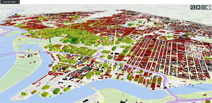
Buildings are colored by height. For this snapshot of the neighborhood, north is rotated ~30° to the right. Rivers shown are the Anacostia (left to right) and the Washington Channel/Potomac River (left side). Shorter buildings are colored black to red, while taller buildings are shown in shades of green. (This figure is visualized in Cesium83 using Open Data DC58 building input. An interactive version of the figure can be found at: bit.ly/IM3_DC_99).
Initial comparisons of model output to observations
To evaluate the model performance in comparison to observations, we first show daily average temperature and relative humidity comparisons over the 10-day heat wave at two locations, Reagan National Airport (DCA) and the National Arboretum. Because relative humidity measurements were not available at the Arboretum location, we also include 1 km Daymet reanalysis (see section “Methods” for Daymet description) output for comparison at both locations. The reason only two measurement locations were compared to model output is that those were the only two measurement stations in the area that had archived data for 2010. However, we note that NOAA Air Resources Laboratory (ARL) has begun a revitalization of its rooftop meteorological measurement towers in Washington, DC (previously DCNet, now UrbanNet) by upgrading and expanding that building-scale measurement network37. We look forward eagerly to the availability of validation measurements from UrbanNet for future studies of this area.
The simulation output used in the comparison is the model output at the grid cell containing each measurement site. Figure 2 shows that grid cell values of the simulated daily average temperature track well with the DCA measurements for the first four days, then stay below observations until day 10. The largest difference between the measurements and the simulations is about 9 °F (5 °C) on day 7. Simulations using 3D morphological input (similar enough that results plot on top of one another) show slightly higher average temperature (closer to observations) during days 6 and 7, the hottest days of the heat wave, but dip lower than the simulation run with no morphological input until day 9. All simulations spike upward at day 10. Simulated temperatures at the Arboretum follow a similar pattern to those output for DCA, but they track above the measured temperatures at the Arboretum. Results from the simulations using 3D morphology plateau from day 4 to day 5, then are similar to Daymet (2-5 °F (1–3 °C) higher than the observations) through day 6. As in the DCA case, all simulations dip similarly downward until day 9 and spike upward at day 10. We note that in both measurement locations, there is no coverage by NUDAPT, and that DCA is not covered by the 10 m and 100 m morphological inputs. (See Supplementary Fig. 1) for comparisons of land cover urban fraction and urban parameter coverage and values.) Average Daymet temperatures are as much as 6 °F (3.3 °C) lower than those at DCA and are within 1–2 °F (0.5–1.1 °C) of those at the Arboretum through July 8 and then are up to 6 °F (3.3 °C) higher for the remaining three days.
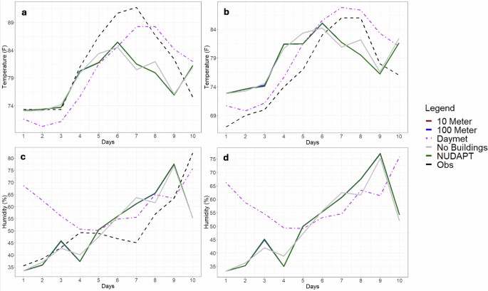
a DCA temperature, b National Arboretum temperature, c DCA relative humidity, d National Arboretum relative humidity point value comparisons at the grid cells containing each of the measurement locations simulated with WRF using 10 m (red line) and 100 m (blue line), NUDAPT 1 km (green line), and no (gray line) morphology inputs for the Washington, DC area for 1–10 July 2010. Observations are shown in black (dashed line). Daymet grid cell daily values are in magenta (dot-dash line). Temperature observations from the National Arboretum, in this case, are for observations that occurred sometime during each day between the minimum and maximum temperatures, but are not necessarily averages.
Simulated average relative humidity tracks within 2.5% of measurements at DCA for the first three days, with simulations run with 3D morphological inputs overestimating relative humidity at day 3. All simulations drop below observations on day 4 with the no building input 9% below observations and the simulations including morphology 11.5% below observations. At day 5, simulations using morphological inputs begin to overestimate the relative humidity and remain high through day 9. The no building simulation exceeds observations by day 6 and remains high through day 9. The largest differences occur on day 7 at 15% and 18% with and without morphology, respectively. Average humidity simulations drop well below measurements by day 10 (−27.5%). Daymet values are similar to measurements on days 4 and 5 but show little agreement again until day 9. Values from the WRF simulations at the Arboretum location are similar in trend to but track higher than those of Daymet between days 5 and 8. By day 9, the simulation using no morphology shows relative humidity 13% points higher than Daymet and the simulation using morphological inputs 15% points higher.
Some of the bias observed in the simulation outputs may be due to the sensitivity of the model to the difference in the urban terrain between that which would have been present in 2010 and that which was used (2015) in the model simulation38. However, we note here that systematic cold bias and overestimation of humidity during the summer is generally characteristic of the WRF model39,40,41. In particular, the summer cold bias in the WRF model has been attributed to large overestimation of surface albedo42 and to overall underestimation of entrainment39. Additionally, simulations performed for the study here used the BouLac43 planetary boundary layer (PBL) scheme. We note that PBL scheme experiments by44 testing Mellor-Yamada45 and BouLac length scales at three resolutions in the 250 m–1 km “gray zone” show a cool bias associated with BouLac length scales throughout the PBL column as compared to large eddy simulations (LES) for the same horizontal resolutions. However, the BouLac based results were less grid-scale dependent with respect to heat transfer between the surface layer and the PBL column than the Mellor-Yamada-based results. A comparison of Supplementary Fig. 3 with Fig. 2 shows a comparable similarity across resolutions with this set of simulations. To minimize the temperature bias, we configured WRF to match that with the least summertime low bias reported by46 that tested the sensitivity of simulated 2-m temperature to a variety of different WRF configurations (see section “Methods”).
Differences in wind speed and direction among observations and simulations are shown in Supplementary Fig. 7. We note that the southerly winds are underrepresented in the simulations because we did not set WRF up to read in the building roughness length parameter values from our input files, nor did we use any of the predefined BEP urban classes. As a result, the roughness length used was what we believe to be a “mosaic” value (0.14 m) because the calculated 2D urban fraction in each cell was less than 1 in every case. Because this mosaic value is much lower than realistic roughness lengths for even low-rise residential areas and much lower than those calculated for the summertime forested areas in the southern part of the domain (some of which erroneously overlap the Potomac River), we hypothesize that the resulting wind characterization was based on an overestimation of the impact of vegetation roughness lengths on wind speed and direction and an underestimation of the urban canopy contribution (see Supplementarly Fig. 2, panel (b) for distribution of roughness lengths in the domain).
Hourly biases for temperature, relative humidity and wind are shown in Supplementary Fig. 9 and Supplementary Table 5. Cross-simulation comparison of spatially-averaged daily maximum average and minimum planetary boundary layer height is presented in Supplementary Fig. 8.
Spatial visualization and comparison
Because the spatial distribution of each resolution’s urban parameter inputs differs from the others across the study area (Supplementary Fig. 1), we expected the distribution of the simulations’ meteorological outputs to differ spatially as well. We expected this especially because the main contribution that 3D urban parameters make to the Building Effect Parameterization (BEP) urban physics scheme used in these simulations47 is the layer-by-layer (for 15 vertical layers) weighted averages applied to the heat and momentum exchanges calculated by the PBL scheme. To visualize this heterogeneity in temperature during the heat wave for each simulation, we averaged the 2m temperature outputs in each 270 m grid cell over the 10-day period. Figure 3 shows the resulting spatial distribution of the 10-day average temperature outputs over the 2010 heat wave for each of the four simulations.
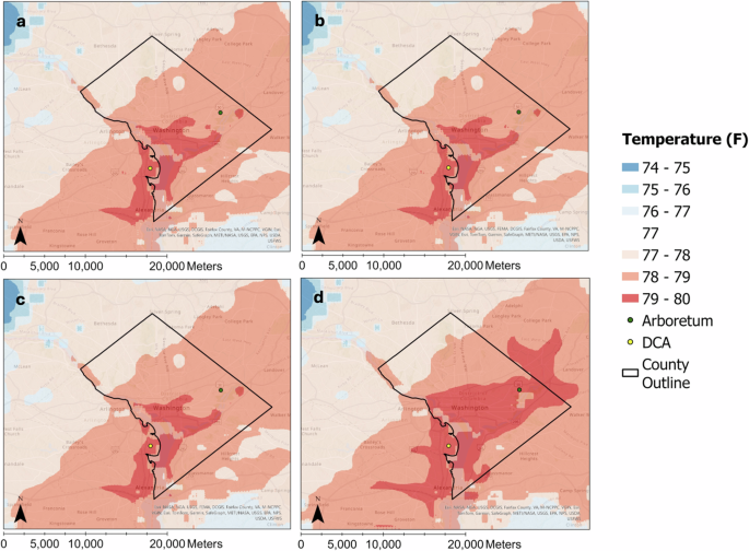
a 10 m, b 100 m, c NUDAPT 1 km resolution morphologies, d no urban morphology for Washington, DC run with 1–10 July 2010 meteorological initial and boundary conditions. Green (Arboretum) and yellow (DCA) points show the point locations of the measurement stations used for validation.
Temperature differences across the domain for all simulations span ~7 °F (4 °C). All figures show a wide orange band of area one degree F lower than maximum running southwest to northeast across the county over the most densely urban portion of the county. All figures also show the maximum average temperature (red) just northeast of the Potomac and south of the Arlington National Cemetery greenspace. The maximum average temperature covers a much larger area in the visualization of the results of the simulation run with no morphological inputs (panel (d)), including the poorer neighborhoods southeast of the Anacostia River. Simulations run with the 10m and 100m resolution morphological inputs (panels (a) and (b)) show average temperature coverage that is nearly identical, while the simulation run with NUDAPT (panel (c)) shows slightly less coverage of the maximum average temperature in the area just north of DCA (yellow dot). The simulation run with the 10m resolution shows maximum average temperature an additional small neighborhood southwest of the Arboretum (green dot). All simulations use the same 2D urban land cover, and this likely accounts for the overall similarity among the outputs. Additionally, where 3D building input information is absent, as it is outside the DC county boundary, urban parameters are taken from the URBANPARAM.TBL lookup table48. Prescribed heights of buildings in grid cells identified as “urban” in the land class maps are treated in the proportions defined as “high density residential” by the BEP scheme. Supplementary Fig. 2 (panel a) shows the landcover characteristics for the domain. For values outside the DC boundary, all simulations used the same prescribed grid cell landcover characteristic values. 10-day maximum temperatures, shown in Supplementary Fig. 4, display much higher variation across the city. Additional figures showing spatial distributions of meteorological variables can be found in the Supplementary Figs. 5 and 6. In summary, the simulated results show various locations across Washington, DC up to 3 °F (1.7 °C) warmer or cooler, 8% points wetter or drier, and 2 ms−1 windier or calmer depending on the resolution of the morphology used in the simulation.
Analysis of spatial differences among simulations
To quantify the differences in spatial heterogeneity seen in the 10-day averages of each heat wave related variable in each 270 m grid cell of the simulations run with no buildings, the NUDAPT 1 km morphology, and the 10 m and 100 m morphology inputs, we computed a set of summary statistics (Supplementary Table 2) and performed Mann–Whitney U tests comparing results from the simulation using 100 m inputs to the those of the other three simulations (Table 1). Samples for these tests included 10-day averages of temperature, relative humidity and wind speed at each 270 m grid cell of each of the four simulations. 10-day averages of sensible (SH) and latent heat (LH) values were also evaluated for the simulations to gain further insight into the energy balance at neighborhood scale and its impact on neighborhood temperature, humidity and wind. Three of the input urban parameters were also compared using this test: the building plan area density (Build_Area_Frac), the building height weighted by building plan area (Build_Height) and the building surface to plan area ratio (Build_Surf_Ratio).
The Mann–Whitney U test is a non-parametric test that compares two groups of data to determine if the groups are sampled from populations with identical distributions. Here, the null hypothesis is that each of the 10-day averaged variable values in each 270 m grid cell in Washington, DC run with the 100 m morphology (Simulation A) are sampled from identical distributions as their counterpart 10-day averaged variable values in the 270 m grid cells run with each of the 10 m morphology, the NUDAPT 1 km morphology or with no morphological input (Simulations B). Stated another way, this is the probability of randomly selected values of each variable from Simulation A being larger than those of each variable from each Simulation B is equal to that of those output from each Simulation B being greater than those output from Simulation A. P-values <0.05 in this case indicate that the null hypothesis is rejected and the variable values are not sampled from identical distributions. The “W” statistic, the large numbers shown in Table 1, is calculated for each variable by comparing its 10-day averaged value for each 270 m grid cell run with the 100 m resolution (Simulation A) morphology to the corresponding 10-day averaged value for each 270 m grid cell run with each of the 10m resolution, NUDAPT and no morphological input simulations and determining which of the values in each pair is greater. The number of times the values from the simulations using the 100m morphology Simulation A are greater than those of the Simulations B are tabulated and presented as the W statistic. For each simulation, variable values from 12,000 grid cells were used, so to calculate the W statistic 12,000 × 12,000 = 144,000,000 comparisons were made for each simulation pair. Thus, if the value of the W statistic is near 72,000,000 (half the number of comparisons made), the distributions from the simulations run with the 100 m resolution and the simulations run with, e.g., the 10 m resolution are similar. If the W statistic is greater than 72,000,000, the result shows that the simulation using the 100 m resolution morphology produced higher values than those run with the 10 m resolution morphology more often than 50% of the time. If the value of the W statistic is lower than 72,000,000, the result shows that the simulations using the 100 m resolution morphology produced lower values than those run with the 10 m resolution.
As shown in Table 1, the null hypothesis, that each of the 10-day averaged variable values in each of the 12,000 270 m grid cells run with the 100 m morphological inputs (Simulation A) are sampled from an identical distribution to their counterpart 10-day averaged variable values (Simulations B) run with 10 m and NUDAPT morphological inputs is upheld, but is rejected for the simulation run with no morphological inputs for all variables tested (p < 0.001). The W statistic shows that spatially, for average temperatures, the values produced by the simulation with no morphological inputs were higher for more than half of the 12,000 270 m grid cells. For average relative humidity, values were lower, and for average wind speed they were higher. For average sensible heat fluxes, the simulation with no building input values were lower for more than half the grid cells and for average latent heat fluxes, values were higher. Averages for latent and sensible heat used signed results rather than absolute values and do not capture the direction of the fluxes.
For comparisons of three urban parameter inputs, building area fraction, building height and building surface ratio, the 100 m resolution morphological inputs showed higher values than those of any of the other three resolutions. (Full set of urban parameters calculated are in Supplementary Table 1 and spatial visualization of the building heights at each resolution can be found in Supplementary Fig. 1. Summary statistics for the three urban parameters evaluated here can be found in Supplementary Table 3. We note that of the 132 urban parameters generated, only the plan area fraction, the area-weighted mean building height, the building surface to plan area ratio, and the distribution of building heights are used by WRF for these simulations.) The main conclusion we draw here is that taken as a whole, the 10-day average meteorology generated in each simulation is distributed similarly among the simulations using 3D morphological input, but differently from that of the simulation using no morphological inputs.
Application to sustainability and energy justice
Records beginning in the late 1800s for Washington, DC show that its population has grown continuously, and that its land surface radius has expanded with greater heat-absorbing paved and built area leading to increasing heat records within the city and intensifying its urban heat island effect49. During the summer of 2010, Washington, DC recorded temperatures that surpassed 98 °F (37 °C) on 11 days, reaching a peak of 102 °F (39 °C) on July 6 and 7. July 6 of that year broke two records: the earliest 100 °F reading in a day, occurring before noon, and the longest uninterrupted stretch of temperatures above 100 °F (7 h). However, while record highs during the day may capture headlines, heat waves produce their greatest impact with high night time minimum temperatures, as heat is essentially trapped in the urban core during the day rather than escaping into space49. Consequently, many urban residents do not recover from the daytime heat, increasing their vulnerability to heat-related illness over subsequent days50. The 2010 and 2011 heatwaves in Washington, DC produced both the most and the second most nights above 80 °F (7 in 2011 and 4 in 2010) in the historical record49. It is on two night time hours associated with these record high minimum temperatures, July 6 and 7, that we focus this section.
Because one of the aims of this paper is to understand how differences in the resolution of model inputs might change the understanding of how a heat wave affects the most vulnerable populations in the city, we used model outputs to calculate the heat index by U.S. Census Tract for the identified night time hours in shown in Fig. 4. For both hours, the heat index displayed is lowest across the city for the simulation using no morphological inputs. Differences in the heat index on July 6 at 5am among the three simulations run with morphological inputs are found mostly southeast of the Anacostia River in 2010’s two lowest income wards51, Wards 7 and 8. Output from the NUDAPT simulation shows three large census tracts and one adjoining smaller one with a heat index of 82–83 °F (45.5–46 °C), a linear stretch of tracts just southeast of the Anacostia with a heat index of 84–85 °F (46.7–47.2 °C) and the remaining area of the two wards at 83–84 °F (46–46.7 °C). For the simulations run using the 10 m and 100 m morphological inputs, an additional census tract is included in the linear stretch of tracts with the highest heat index, and the larger of the two adjoining tracts with heat index of 82–83 °F (45.5–46 °C) in the NUDAPT simulation is at a heat index of 83–84 °F (46–46.7 °C) in the 10 m and 100 m simulations.
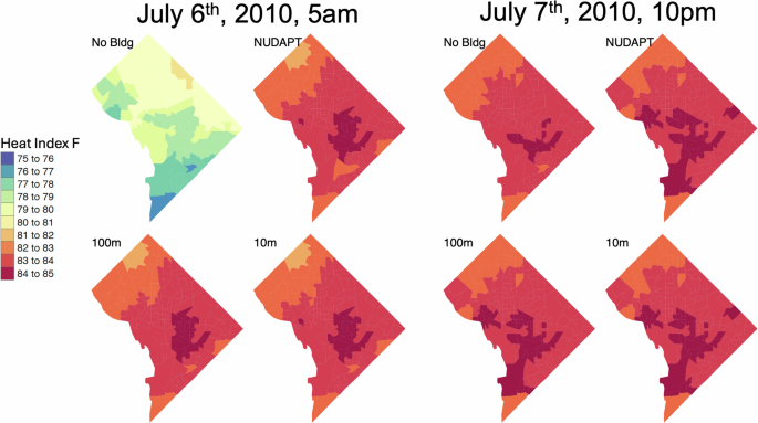
The No Bldg panels show heat index calculated using output from the simulation with no 3D building input. The NUDAPT panels show heat index calculated using output from the simulation containing the 3D NUDAPT 1km input. 100 m and 10 m panels show heat index calculated from the output of simulations using 100 m and 10 m 3D morphological input, respectively.
For the July 7 10 p.m. hour, the heat index is 82–85 °F (45.5–47.2 °C) across the city for all simulations. For the simulation using no morphology, only a small x-shaped set of census tracts shows the highest heat index, and the heat index of the entire northwestern part of the city is at the low side of the range. All simulations run with morphological inputs show much larger areas of the highest heat index. That run with the NUDAPT input shows the largest number of tracts at the highest value.
Results from population-weighted regressions quantifying the association between heat exposure and social vulnerabilities (see Methods section “Sustainability and energy justice”) show substantial dependence on the vulnerability characteristics used, and some dependence on the resolution of the input data used in the WRF simulations. Across all outputs of the WRF simulations, tracts with higher shares of the population characterized as vulnerable by the Centers for Disease Control (CDC) based on their socioeconomic status52 show a statistically significant positive association with heat index (Table 2) and with temperature (Supplementary Table 4). Working through Table 2, we note that for all simulations, Census tracts with a socio-economic status based social vulnerability index were positively correlated (0.71 to 0.78) with the heat index on 7 July 2010 at 10 p.m. Tracts with vulnerability due to household characteristics showed negative correlation with heat index (-0.47 to -0.32 ). Tracts with high vulnerability due to racial or ethnic minority status (or who speak limited English) also had a statistically significant negative association with heat index (-0.63 to -0.41). times No significant relationship regarding heat exposure was seen among tracts more or less vulnerable due to housing type and transportation.
Figure 5 displays the difference in regression results for each social vulnerability index using output data produced by each of the four WRF simulations for 6 July 2010 at 5 a.m. The differences in these results among the 10 m vs 100 m vs 1 km (NUDAPT) resolution building inputs are not statistically significant. However, for socioeconomic vulnerability, the regression performed with heat index results from the simulation using no buildings showed a negative correlation of socioeconomic vulnerability and heat index, whereas results from the simulations using 3D building inputs showed a positive correlation between socioeconomic vulnerability and heat index. Additionally, while heat index values calculated from simulation results using 3D building inputs showed a small negative correlation to race, ethnicity and language vulnerability, heat index values calculated from simulation results without 3D building inputs showed a strong positive correlation to vulnerability associated with race, ethnicity and language. A similar summary of regressions for 7 July 2010 at 10 p.m. using temperature as the dependent variable is shown in Supplementary Fig. 10.
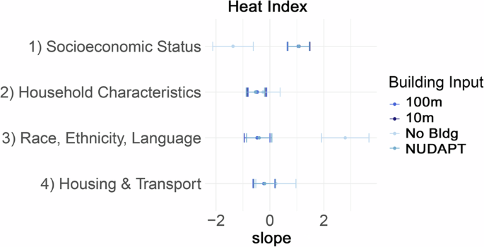
Regression with each SVI as the independent variable and Heat Index as the dependent variable for 6 July 2010 at 5 a.m.
Discussion
We have shown that for WRF simulations at 270m horizontal grid spacing over the city of Washington, DC, the spatial variability in temperature, humidity, wind speed, wind direction, and sensible and latent heat fluxes across the city can vary slightly with the resolution and the coverage of the 3D urban morphological input, but that larger differences occur between simulations run without morphological input and those run with some type of morphology. We have also shown that the variation in heat index during a heat wave over a city during hours of minimum temperature can produce differences in calculated impact on vulnerable populations. In this study, the differences we report occurred mostly over the locations of 2010’s lowest income neighborhoods in Washington, DC. We do not ascribe any socioeconomic cause and effect to this result, we only note that some modeling discrepancies can arise in city locations where results may matter most for neighborhood-level assessments. We did not find the large spatial differences among simulations run with 3D input morphology at different resolutions that we expected we would find, in part because the urban areas outside the boundary in which we provided urban parameters made up a large part of the domain, and were parameterized the same way in all simulations, and partly because we did not include input-building-defined roughness length calculations in the simulation. However, we did identify some of the contributors to differences in spatial heterogeneity of the heat wave among the simulations, note small neighborhood discrepancies between results using the lower-coverage NUDAPT inputs and the higher coverage inputs at higher resolution, and quantify some of the uncertainty around the simulation results.
Researchers and urban planners have begun to develop future scenarios, pathways and plans, and to implement projects that improve urban resilience and sustainability53. Awareness of the initial assumptions, model input implications, and the overall uncertainty in these analyses is important to urban resilience and sustainability planning especially as average and extreme temperatures continue to rise in the future. As street-level meteorological data continues to be collected and archived for major cities, it will be instructive to learn how these higher resolution observations compare with model results5. Likewise, as additional parameters are integrated into the urban morphological input data for models, such as custom roughness lengths, and eventually custom building roof radiation, thermal conductivity, heat capacity, and emissivity54,55,56, additional feedbacks between the built environment and the natural environment can be simulated at the most appropriate resolutions to the scientific questions under investigation.
Methods
Model domains and parameterization inputs
Four 1-month, three-domain, nested meteorological simulations were conducted using WRF Version 4.2.1 for the month of July 2010 using North American Regional Reanalysis (NARR) data57 as initial and boundary conditions. Three of the simulations were run using urban morphological parameter inputs; the fourth was run with no morphological parameters. The resolution of the morphological inputs were 1 km (NUDAPT) 100 m and 10 m (the latter two input sets calculated using Python code developed by the researchers (described in the next paragraph)). The simulations, centered on the city of Washington, DC used the WRF model run on the Oak Ridge National Laboratory (ORNL) Compute And Data Environment for Science (CADES) supercomputer. The horizontal resolution for each of the model domains (from outermost to innermost) was 6750 m (d01), 1350 m (d02), and 270 m (d03) with 99 × 93, 145 × 135 and 100 × 120 grid cells, respectively (Fig. 6). Each domain contained 43 vertical levels with the model top at 100 hPa.
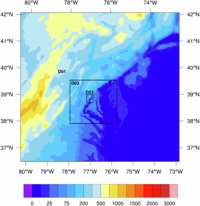
The innermost domain is centered on the Washington, DC Waterfront neighborhood. The colorbar shows the natural terrain elevation of the location in meters.
The urban morphology inputs at 10 m and 100 m resolution were generated using a 1m resolution shapefile of building footprints from 2015 and corresponding building heights acquired from Open Data DC58 for the year 1999. Because building heights were not available for the 2015 footprints, the above-surface meteorology in this experiment is affected primarily by the 1999 morphology. From the Open DC shapefile, urban parameters were calculated for 15 vertical levels at 5m intervals following the methodology of the NUDAPT project13 and fulfilling the criteria for the WUDAPT22 “L2” data. Supplementary Table 1 shows the parameters calculated. Parameters 1-101 are defined by59, while the skyview factor is calculated based on60, the Grimmond and Oke roughness length and displacement height use the61 equations, Raupach roughness length and displacement height use the62 equations, and the equations for the McDonald et al. roughness length and displacement height calculations are found in63. For the calculation of these parameters, a series of scripts were developed using the Python coding language, which aggregated the 1m resolution building attributes to 10m and 100m resolution to generate the respective urban parameter files as WRF-readable binary files integrable with WRF using the established NUDAPT paths in the WRF simulation environment. Selection of GEOGRID.TBL interpolation options for the 10m and 100m resolution morphological inputs used the resolution of the input data and nearest_neighbor interpolation so that the parameters were resolved during pre-processing at the resolution of the input. For the simulation using NUDAPT, the default:nearest_neighbor option was used.
Landcover characteristics used were obtained from the US Geological Survey 2011 National Land Cover Database (NLCD)64 at 30 m resolution and included in the WRF pre-processing geography input package. The NLCD input provides urban land classifications such as percentage impervious surface, percentage of various vegetation coverage, percentage of coverage of constructed materials and percentage of open water. The impervious surface coverage of each grid cell is particularly important for this study because impervious surfaces contribute to the energy dynamics of urban areas, especially with regard to increased storage of sensible heat, and decreased evapotranspiration65. There are four classifications for impervious surface coverage for each 30m grid cell in the NLCD data set derived primarily from remotely-sensed imagery: developed open space (less than 20% of total land cover is impervious), developed low intensity (a mix of vegetation and constructed materials–impervious surfaces account for 20–49% percent of total cover), developed medium intensity (50–79% of the grid cell is impervious), and developed high intensity (over 80% of the grid cell is impervious). While the land cover characteristics represent well the density of the impervious surface to the model, these characteristics are only representative of the two-dimensional ground surface. The urban morphological parameters described in the previous paragraph are required for the representation of the height variability of the impervious urban area.
The timestep used for the outermost (6750m) domain was 10 seconds. The timestep for each nested grid was in the same ratio to the outer domain as was its spatial dimension. Nesting ratios for the simulations were 5:1. This ratio is based on recommendations from ref. 66 to align U and V velocities calculated at the edges of the parent-to-child Arakawa C-grids with mass quantities calculated at the centers of these cells. The simulations were run from 30 June through 21 July 2010, and each included a 24-h model spinup before the 10-day period evaluated here.
Physics packages for WRF were chosen based on optimum packages for urban scenarios and on a sensitivity test performed by ref. 46. The microphysics package for all domains was Thompson aerosol aware, and the long- and short-wave radiation physics packages used were Dudhia RRTM. The Betts-Miller-Janjic (BMJ) scheme for cumulus physics, the Monin-Obukhov surface physics, and the BouLac planetary boundary layer (PBL) scheme were used for all domains. The BouLac PBL scheme was chosen for these simulations because it is one of two PBL schemes specifically recommended67 for simulations using the Building Environment Parameterization (BEP) scheme (discussed in the next paragraph) and because it has been used successfully extensively with the BEP scheme [e.g., refs. 68,69,70]. Noah-LSM was used for the land surface in all domains.
The urban physics packages chosen were the Single-Layer Urban Canopy Model (SLUCM)71, which calculates surface effects for roofs, walls and roads for the outer two domains; and the BEP scheme72, a multi-layer urban canopy model that allows for input of externally calculated urban parameters (including those pertaining to buildings higher than those at the lowest model levels) for the innermost (270 m) domain in each simulation. SLUCM was chosen for the outer two domains because the urban parameters calculated at 10 m, 100 m and 1 km NUDAPT for the inner domain were for the city of Washington, DC only and not for the area covered by the outer two domains. Additionally, in SLUCM both natural and impervious surfaces are represented to the model and coupled to Noah-LSM through the urban fraction parameter, whereas if the BULK parameterization had been used for the outer domains, the entire urban region in those domains would have been assumed to be impervious73,74,75.
WRF output was postprocessed so that its Coordinated Universal (UTC) timestamps aligned with local Eastern Daylight time for comparison with observations (2 m temperature, relative humidity and 10 m wind) at local time from the archives accessed for both the Weather Underground data reported for the Reagan National Airport (DCA)76 located at {38.85, -77.04} and the National Centers for Environmental Information archives77 for the National Arboretum located at {38.9133, -76.97}. Additionally, 10m windspeed and direction were derived from WRF output of U and V, and relative humidity was calculated using 2m temperature, surface pressure and 2 m water vapor mixing ratio inputs to the NCAR Command Language (NCL) relhum function based on78. Simulation results were compared as well to point values of average temperature and daily vapor pressure converted to relative humidity obtained from the 1km reanalysis dataset, Daymet (Version 3)79. The Daymet algorithm calculates parameters for each of its 1 km × 1 km output grid cells based on the coordinates of each grid cell’s centroid. The surface elevation used at the centroid is the average of the elevation values within in each grid cell included in the National Aeronautics and Space Administration (NASA) Shuttle Radar Topography Mission (SRTM) 30 arc second digital elevation model (Version 2.1)80 over the 1 km × 1 km region.
Sustainability and energy justice
Hourly relative humidity and hourly temperature were used to calculate the heat index for each 2010 census tract using the U.S. National Weather Service81 equations and recommended adjustments according to82. Grid cells and portions of grid cells intersecting each tract were averaged proportionally for each of the four modeled products: no buildings, NUDAPT, 100 m, and 10 m resolution buildings. Results are shown in Fig. 4.
A suite of population weighted regressions were then performed between 8 possible independent variables: temperature and heat index for each of the four building resolution inputs. Each of the 8 independent variables is regressed on the four topical themes in the CDC’s 2010 Social Vulnerability Index. The specific factors that contribute to each theme are shown in Supplementary Fig. 11.
The regressions take the form shown in Equation (1), where HI is Heat Index, i denotes the census tract, α is the intercept, β1 − β4 are regression coefficients, V1 − V4 represent the four themes of the CDC’s 2010 Social Vulnerability Index, and ϵ represents a tract specific error term.
α and β1 − β4 are estimated using weighted least squares where each tract is weighted by 2010 population. There are 179 tracts in the District of Columbia, but 7 are missing SVI Theme 1 data and are thus excluded from analysis. This excludes 19,217 people, (3% of the total population). The same method is applied to assess the association between SVI and Temperature, and using modeled weather dependent on each the four possible building inputs.


Responses