Simulating flood risk in Tampa Bay using a machine learning driven approach
Introduction
Flooding is a common disaster around the world1,2,3, having enormous detrimental impacts on society4,5. The frequency and intensity of floods are rising due to climate change and the consequential damage is dramatically increasing as a result of elevated exposure6. A great amount of research is focused on risk assessment and mitigation strategies7,8. Flooding, as a natural disaster influenced by numerous factors, is challenging to prevent entirely. However, the effects can be significantly reduced through the implementation of risk mitigation strategies9 including by providing risk decision-makers with relevant, accurate risk assessment information that can aid in establishing effective emergency management protocols and communicating with the public to save lives and property. With the increasing frequency and intensity of flooding, it has become imperative to mitigate flood risks effectively. It is thus vital to first accurately assess flood risks. Flood risk assessment contributes significantly to managing floods effectively. These assessments enable us to identify possible threats at both the global and local levels, providing vital information for mapping high-risk areas. This vital information serves as input to targeted interventions, enabling more efficient and effective mitigation and management of flood impacts10. The interaction between naturally occurring events and vulnerable populations leads to complex challenges, specifically, as does the need for different types of authorities and decision-makers to have information relevant to the flood risk decisions they make11 (e.g., when to deploy specific resources during a flood event versus comprehensive planning in advance of a forecasted event). Flood risk assessment is accordingly a multifaceted process encompassing the hazard engendered by naturally occurring events and the social determinants that affect how these events impact human communities12. Researchers have long called for an integrated approach that considers both physical dimensions (hazard and exposure) and social dimensions (vulnerability)13,14,15. An integrated approach to flood risk assessment that includes both physical and social aspects serves as a foundation for policy recommendations and loss minimization14.
The core task in flood risk assessment is to identify the vulnerable locations to flooding to assist sustainable flood planning and prevent losses16. High accuracy in the identification of flood-risk zones has a positive correlation with effective flood risk mitigation17. Flood risk assessment often integrates topological factors, hydrological factors, socioeconomic factors, and climate change impacts into one analytical framework. Integrating these factors into flood risk assessments can lead to the development of better-informed floodplain management strategies, disaster preparedness plans, and infrastructure investments that prioritize the needs of vulnerable communities. Vulnerability can be significantly increased if a system or community is more exposed to a particular hazard. Additionally, their degree of susceptibility and capacity for adaptation or recovery are also deeply connected to their vulnerability12. Understanding the interaction among flood hazards, exposure and vulnerabilities is thus essential for building resilience and mitigating the potential consequences of flooding in the dynamic and at-risk region. Flood risk assessment for mitigation purposes existed long before the data science boom of the past decade. However, recent technological advancements have made this research increasingly popular and practical for effective risk mitigation16,18. Geographic Information System (GIS) and Remote Sensing techniques serve as essential tools to analyze and integrate flood-related information19. Integrating machine learning (ML) classification approaches into the flood risk assessments will offer better prospects of improved accuracy, shorter computation times, and reductions in the overall expenses associated with model development20. Numerous studies have used ML algorithms to assess flood risk8,16,18,21,22,23. Several researchers have explored the application of ML models and decision-making algorithms for flood risk assessment, hazard mapping, and vulnerability assessment, by employing various techniques such as random forest (RF), support vector machine (SVM), neural networks, and logistic regression to analyze flood factors24,25,26,27,28,29.
Despite these advancements, no studies have yet considered past flood damage data and a wide variety of flood risk factors (FRFs) from both physical and social dimensions using advanced ML models to simulate flood risks. Hence, the present study offers three novelties. First, this study introduced a unique approach of assessing flood risk by utilizing past flood damage data as a target variable and a diverse range of FRFs from hazards, exposure, and vulnerability components of flood risk as predictors. This approach can yield robust and more accurate results as demonstrated by Yarveysi et al.30 and Dey et al.29. Based on an extensive literature review, nine hazard factors including elevation, slope, aspect, curvature, precipitation, normalized difference vegetation index (NDVI), distance from waterbodies, topographic wetness index (TWI), and drainage density, and three exposure factors, namely, building footprint density, road network density, and normalized difference built-up index (NDBI) and, four vulnerability factors such as median income, percentage of Hispanic population, percentage of Black (African American) population, and percentage of people with no school completion were used as FRFs. Second, this study examines how accurate the ML models are in predicting flood risk and further compares the simulated flood risk maps (FRMs) with the Federal Emergency Management Agency’s (FEMA’s) 100-year floodplain map. Third, this study highlights some additional uses of ML models in flood risk assessment, aiding policymakers in flood mitigation by identifying key FRFs and vulnerable populations and their locations based on historical flood damage in Tampa Bay.
To implement our analytical strategies, Tampa Bay, Florida in the USA was selected as a test bed. Tampa Bay is located on the Gulf Coast of Florida (Fig. 1), and the area has a population of over three million, according to the 2020 Census. The coastline’s location and proximity to the Gulf make the region vulnerable to extreme weather events. According to the urban adaptation assessment data from the University of Notre Dame, Tampa Bay is exposed to the risk of flooding and sea level rise. Studies have revealed that different communities in Tampa Bay are highly vulnerable due to sea level rise31,32. In the past decade, several hurricanes have passed Tampa and devastated places close to Tampa Bay. Hurricane Idalia (Category 3) landed on the north coast of Tampa, and Hurricanes Ian and Irma, both Category 4, landed on the south coast of Tampa. These events brought heavy rainfall, human casualties, and substantial damage to the economy. The historical average cost of flood events between 2011 and 2015 was over $500 thousand, and the projected cost due to sea level rise is over $700 million by 2040. Considering the significant recent history with flooding and its sizable population, it is an ideal study location for us to test our methods of assessing flood risk using advanced ML algorithms.
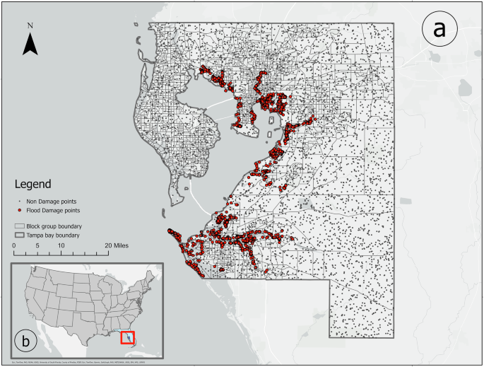
a Boundary of Tampa Bay with flood damage and non-damage points. Red dots indicate the flood damage points while gray dots indicate non-damage points. b The location of Tampa Bay and Florida State in the context of CONUS. This map was generated in ArcGIS Pro 2.4.0.
Results
Models’ accuracy assessment
The process of evaluating the ML models has two major parts. First, all these ML models were evaluated by the AUC–ROC curve (Fig. 2). Later, several evaluation metrics including overall accuracy, precision score, recall score, F-1 score, Kappa score, and Jaccard score were examined to further evaluate the accuracy of these ML models (Table 1).
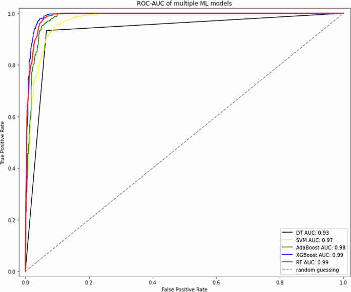
The X-axis represents the false positive rate (1 – specificity) and Y-axis represents the true positive rate (sensitivity). The red, blue, green, yellow, and black lines represent the AUC curves for the RF, XGBoost, AdaBoost, SVM, and DT models, respectively. The gray dotted line indicates the AUC curve for random guessing. This analysis was conducted and plotted using roc_curve function in Python 3.11.7.
According to the ROC–AUC curve analysis, the XGBoost and RF model achieved the highest AUC score of 0.99. On the other hand, the AdaBoost model achieved the second-best AUC score of 0.98. Meanwhile, SVM and DT yielded the lowest score among the models, standing at 0.97 and 0.93, respectively.
The overall accuracy test reveals that XGBoost and RF secured the highest score of 0.96 while Adaboost, DT, and SVM achieved 0.95, 0.93, and 0.92, respectively (Table 1). For precision score, XGBoost secured the best score of 0.94, followed by RF and DT at 0.93, and Adaboost at 0.92, and SVM at 0.87. For recall score, RF achieved the highest accuracy (0.99) compared to SVM (0.98), XGBoost (0.98), Adaboost (0.98), and DT (0.93). The F-1 score for both RF and XGboost were the highest at 0.96 with Adaboost, DT, and SVM at 0.95, 0.93, and 0.92. XGBoost had a Kappa score of 0.93, RF scored 0.92, Adaboost achieved 0.90, while DT and SVM scored 0.87 and 0.83, respectively. For the Jaccard score, XGBoost received a score of 0.93 and RF scored 0.92 while AdaBoost, DT, and SVM achieved 0.90, 0.87, and 0.85, respectively.
Based on the AUC–ROC curve and the results from multiple evaluation metrics, all ML models demonstrated strong performance in flood risk assessment. However, given the slightly better accuracy of the RF and XGBoost models, both were selected to simulate FRMs for Tampa Bay.
Major contributing factors of flood risk
The findings of this study indicate that elevation is the dominant contributor (39%) to flood risk in Tampa Bay followed by distance to the river and waterbodies (25%) (Fig. 3). In addition, building footprint density contributes 7%, road network density contributes 5%, TWI contributes 4%, slope and drainage density each contribute 3%, respectively. However, the rest of the factors have very small contributions.
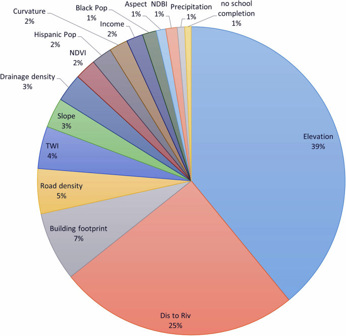
This figure depicts the percentages of contribution of different FRFs in flood risk predictions. This analysis was conducted using feature_importances_ function in Python 3.11.7.
This study further used SHapley Additive exPlanations (SHAP) technique to interpret the importance and contribution of each FRF. These SHAP values not only demonstrate the importance of each feature but also indicate whether their contributions are positive or negative. According to the graph of SHAP method, the regions located in low-lying altitudes are at high flood risks, as flood water naturally flows downward due to gravitational forces and accumulate rapidly from runoff (Fig. 4). Moreover, areas located near waterbodies are inherently more prone to flooding due to the proximity to potential sources of water overflow. Both low elevation and proximity to waterbodies render those coastal regions highly prone to flooding (Fig. 4), especially when heavy rainfall and tropical storms surge cause water to overflow.
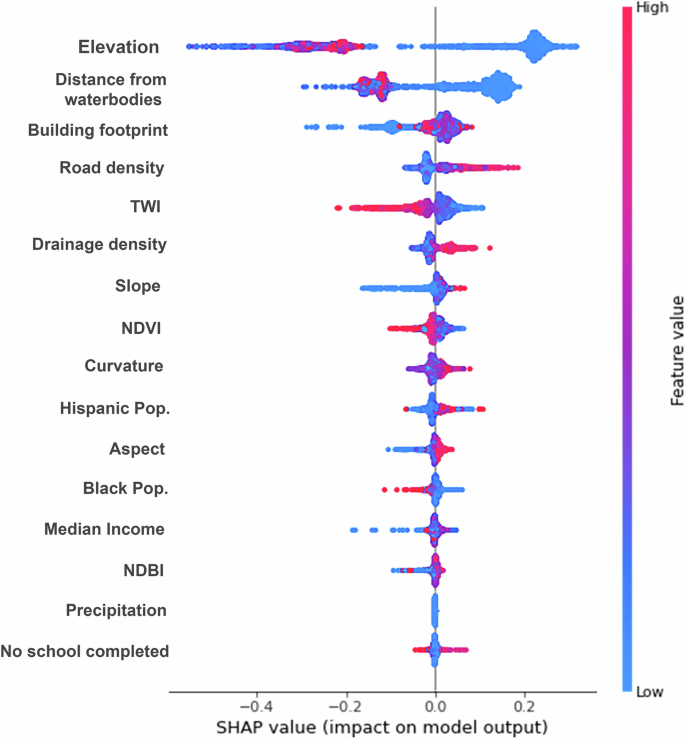
The X-axis displays the SHAP values, where a positive value indicates a higher contribution to flood risk and a negative value indicates a lower contribution. The primary Y-axis lists the names of the FRFs, while the secondary Y-axis shows the corresponding value ranges for these factors. Red dots indicate higher values of FRFs, while blue dots indicate lower values. The plot was generated using shap function in Python 3.11.7.
High density of building and road network increases the risk of flooding, whereas low density reduces this risk for two reasons. Dense man-made infrastructure is often associated with urbanization, which indicates intense human activities such as construction of settlement and thus significant alteration of the land surface. Urban land mostly made up of concrete absorbs water less efficiently for the reason. Meanwhile, a congested community with high buildings and road density suggests increased exposure to hazards. Whenever a disaster strikes, more of the population assets and infrastructure would be susceptible to the devastating impacts. All these conditioning factors have turned out to be prime determinants of flood risk in Tampa Bay.
Considering the contributions of all these FRFs, it can be summarized that geographical location, topographic and demographic conditions of a region highly contribute to amplify flood risk in a region. In Tampa Bay region, densely populated communities located in low altitude near the coast face a particularly high risk of flooding.
Flood risk simulation using RF and XGBoost model
Table 2 displays the distribution of flood risk area in Tampa Bay classified by the RF and XGBoost models. The findings from the RF model indicate that 2.42% of the area of Tampa Bay is at a very high risk for flooding while the XGBoost models classified 3.85% regions at very high risk. These areas are mainly adjacent to Tampa Bay areas which marked as red in Fig. 5.
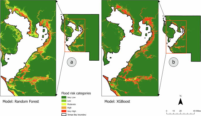
a Flood risk map simulated by RF model. b Flood risk map simulated by XGBoost model. These figures represent the spatial distribution of flood risk zones in Tampa Bay at different levels of risk. Where, green color indicates very low risk, light green represents low risk, yellow color represents moderate risk, orange color represents high risk, and red color represents very high risk of flooding. The simulation was conducted in Python 3.11.7 and the maps were generated in ArcGIS Pro 2.4.0.
In addition, the RF model and XGBoost model classified 2.54% and 1.11%, respectively, of the total Tampa Bay area as high risk, marked in orange color. Furthermore, 2.78% of the area is at moderate flood risk according to the RF model while XGBoost model classified 1.04% areas in the category of moderate flood risk. However, RF model indicates 4.32% regions are at low risk of flood, on the other hand, XGBoost indicates 1.34% areas at low flood risk. The remaining portion of the Tampa Bay is classified as very low risk for flooding by the RF and XGBoost model. These results indicate that both the RF and XGBoost models identify almost similar proportions of areas classified as high and very high risk for flooding. Nevertheless, the RF model exhibits a more detailed spectrum of risk levels compared to the XGBoost model.
Moreover, based on the analysis, it is found that 10.29% of Tampa Bay’s total population are exposed to a significant level of flood risk, falling either into very high or high flood risk categories. Within this group, 13.98% are Hispanic origin and 6.38% are identified as Black population.
Comparing the flood risk map with FEMA’s 100-year floodplain map
Hurricane Irma (2017) was a record-breaking Category 5 hurricane in the Gulf of Mexico and Caribbean Sea. Its maximum storm surge in Florida, USA had a return period ranging from 110 to 283 years33. It generated peak storm surge with a 92–109 year return period in the Florida Keys and 41–254 years along Florida’s Gulf Coast. However, most of the gauging stations in Gulf Coast experienced storm surges with a return period of nearly 100 years during Hurricane Irma33. In addition, the FEMA 100-year floodplain is a key policy tool that directly guides federal flood insurance purchase and mitigation in the USA34,35. So, this study aims to compare the FRM, generated from Hurricane Irma-induced past flood damage data, with FEMA’s 100-year floodplain map for Tampa Bay.
To compare them we overlaid the FRMs from RF and XGBoost models with FEMA’s 100-year floodplain map. It is observed that the high-risk areas identified by RF and XGBoost model coincide with the FEMA’s 100-year flood zones (Fig. 6). All the identified high and very high flood risk areas lay within the boundary of the FEMA’s 100-year floodplain. Meanwhile, our FRM distinguishes from FEMA’s 100-year floodplain map in a critical manner. FEMA’s flood zone designation is binary, determining one area either inside or outside a special flood hazard area (SFHA). This binary designation lacks nuances, leading to inaccurate estimation of flood risks, which further misleads risk mitigation behaviors34,35. Conversely, our flood risk assessment provides a spectrum which can more effectively guide planning and policy-making efforts to prioritize high and very high-risk zones, while the surrounding areas that are categorized as moderate or low risks can be considered with less urgency accordingly. This nuanced understanding can help efficient allocation of resources, especially with strained resources during an emergency.
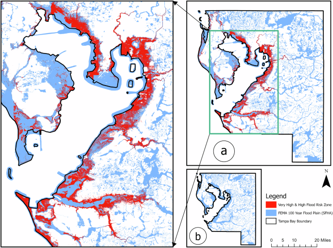
a An overlaid FRMs and FEMA’s 100-year flood plain map. b A FEMA’s 100-year floodplain map of Tampa Bay highlighting special flood hazard area (marked as blue). This map was generated in ArcGIS Pro 2.4.0.
Discussion
In this study, we considered Tampa Bay as a pilot study area, considering various risk factors such as its low-lying topography, coastal location, and history of severe weather events that contribute to frequent flooding. A total of five different ML models, including DT, SVM, AdaBoost, XGBoost, and RF, were trained and tested using flood damage data and FRFs to evaluate the effectiveness of each model in flood risk assessment. This study validated the results with a widely accepted method the AUC–ROC curve and several evaluation metrics including overall accuracy, precision score, recall score, F-1 score, kappa score and Jaccard score. Both the AUC–ROC curve and the other evaluation metrics supported that all ML models performed very well while RF and XGBoost model performed slightly better than others. However, it cannot be conclusively stated that the RF and XGBoost model are the universally superior ML model for other regions around the world. Any variations in the geographical location would result in a different dataset, and the performance of these models would intrinsically depend on the characteristics of that corresponding dataset. In the literature, a few papers established RF model as superior model in flood susceptibility assessment29. While a few other studies found that XGBoost is highly accurate in performing flood hazard assessment23,36,37,38.
Both RF and XGBoost models suggest that nearly 5% of Tampa Bay, especially the areas adjacent to the coast, is at a very high or high risk (Fig. 5). This very high- and high-risk region from both models coincides with FEMA-designed 100-year flood plain (Fig. 6). Different from FEMA’s 100-year flood map, our FRM presents a broader spectrum of risks, including very low, low, moderate, high, and very high-risk zones, providing a nuanced understanding of flood risk to decision-makers. A significant portion of Tampa Bay’s population (10.29%) inhabits this area, among them 13.98% is Hispanic and 6.38% is Black, posing a potential threat to a large community.
Among the 16 FRFs, elevation (39%) was reported as the most dominant factor. This finding is consistent with that of many studies. Specifically, Desalegn and Mulu39 did flood risk assessment in Ethiopia, Ziarh et al.40 in Malaysia, Hoque et al.41 in Bangladesh, Vojtek and Vojteková42 in Slovakia, Dey et al.29 in New Orleans, Louisiana and Mukherjee and Singh43 in Harris County, TX. They all reported that elevation is the most important factor determining flooding. This study also revealed that distance from the river or coast (25%) is the second most important factor for flood susceptibility in Tampa Bay. Many studies reported identical findings44,45,46,47. Communities residing near rivers or coastlines face a substantially higher flood risk compared to those farther inland. This increased risk is primarily due to the combined impact of coastal storm surges and heavy rainfall, which can exponentially escalate the flooding threat during high precipitation or extreme weather events48. Additionally, highly dense built-up areas with dense building and road network was reported as a substantial contributor to flooding in Tampa Bay. Higher infrastructure density increases the exposure of a community and ultimately contributes to escalating flood risks by preventing the natural drainage system of water and reducing the percolation process.
However, the findings indicate that the probability of flood risk is primarily driven by hazard factors (i.e., low-lying areas and proximity to waterbodies) and exposure factors (building footprint density and road network density) while vulnerability-related factors, such as socioeconomic conditions, appear to have less influence. The reason could be that this study trained ML models using flood property damage data. As a result, it makes sense that hazard and exposure factors had seemed the most contributing factors, since property damage is more closely related to hazard and exposure components than to vulnerability. If the ML models were trained using indicators like the flood fatality or death toll data, socioeconomic factors would likely have shown a more significant impact. Future studies could consider using flood fatality data to train the ML models. Despite the limitation, this study adopted state of art methods and incorporated all critical components of flood risk when simulating it. The final visualization of flood risk distribution in Tampa Bay presents a comprehensive FRM.
This identification of areas with flood risk will inform policymakers about the existing condition, which is invaluable for sustainable flood risk management. Without identifying a potential threat, the goal of effective flood risk management is unachievable. Moreover, ML models have identified several very high-risk zones, where the presence of substantial man-made infrastructure significantly elevates the overall flood risk to these communities. If no adequate mitigation measures are taken, these communities will be confronted with increased exposure to elevated flood risks. While the scientific community widely recognizes that elevation, distance from rivers or coasts, and dense urbanization are key factors influencing flood risk, we still advocate for their consideration in specific local flood risk management. These factors are crucial for both risk assessment and mitigation efforts. These hazards, exposure, and vulnerability indicators combined are meaningful variables for flood risk planning because these data are readily available (or likely accessible) to risk decision-makers in their own jurisdictions. This information can be used to develop proactive flood planning measures and mitigation strategies, including public communication and information strategies in heavily populated areas, that are sensitive and specific to the physical and social characteristics present in authorities’ jurisdictions; moreover, flood risk planning and response strategies can be dynamic depending on local, regional, and broader fluctuations in these flood risk predictor variables. Policymakers and planners in the respective areas should consider these factors when planning for and managing flood risks, especially due to likely exacerbations promoted by climate change. Low-lying areas are more prone to flooding9,49. This understanding is important for policymakers for pinpointing areas at high risks of flooding, which will assist them to plan exactly where they should offer intervention for more stringent flood management measures. Informed by factors such as proximity to rivers or coasts, policymakers can enhance land use planning and development by creating flood-resistant infrastructure and enforcing zoning and robust building codes designed for resilience50. They can also strategically allocate resources to establish monitoring and early warning systems and ensure that emergency services are available and accessible in these high-risk areas, increasing the community’s safety and reducing the potential impact of flooding. By considering building footprint and road network density, policymakers can effectively plan timely evacuation protocols and allocate resources in advance, ensuring efficient and successful flood management51.
In the context of global climate change, sea level rise, and increased social vulnerability, disasters are more frequent, and the risk of severe impacts is high. To address this, enhancing community resilience through infrastructural, social, economic, and institutional measures can be an effective flood risk management strategy. This study demonstrates an effective approach to assessing flood risk by considering a wide spectrum of FRFs using advanced supervised ML algorithms. Through this approach, we were able to identify the zones under very high and high flood risks in Tampa Bay, along with the identification of responsible FRFs, in addition to potential exposed populations. Such risk identification procedures will enable us to take precautions and to better prepare for floods at both household and institutional levels. The risk identification is believed to ultimately advance flood resilience. All the findings will contribute to flood risk management both scientifically and practically. The findings can be meaningful in the vast scientific field for flood management studies around the world and the approach will directly assist the policymakers during their decision-making regarding flood risk management.
Methods
Flood risk modeling
To perform flood risk modeling, it is crucial to first define flood risk. Flood risk is defined as the function of the likelihood of a flood event and the potential loss of its negative impact on a community. The Intergovernmental Panel on Climate Change (IPCC) has characterized flood risk as the function of the interactions of three components: hazard, vulnerability, and exposure25,52,53. Hazard refers to the probability of flood inundation and the magnitude of flooding events that are influenced by the natural characteristics of a region. Exposure refers to the presence of population, assets, and infrastructures that are likely impacted by flooding events. Vulnerability refers to the susceptibility of a community or incapacity of a society to deal with the adverse impacts of flooding events. The combination of these three components can provide comprehensive information about flood risk52. Therefore, it is essential to consider causative factors from hazard, exposure, and vulnerability for flood risk modeling of the area. This study aimed to simulate flood risk by considering nine causative factors related to hazard, three causative factors related to exposure, and five causative factors related to vulnerability. These causative factors from three aspects also known as FRF will be the predictor variables. The past flood damage induced by Hurricane Irma as a Category 5 hurricane in September 2017 will be the target variable in the simulations.
Data sources
This study acquired several datasets from different dimensions of flood risk such as hazard, exposure, and vulnerability (Table 3). Majority of the hazards and exposure-related data are secondary or remotely sensed data which were collected from various sources at different spatial resolutions. Census data were collected from the US Census Bureau (https://data.census.gov/cedsci) at block group level. The datasets from both physical and social dimensions were utilized to simulate the FRM. Since they had different spatial resolutions, they were all resampled into a 10 m spatial resolution and converted into GCS NAD 1983 before flood risk simulation.
Methodology
To simulate flood risk using ML models, two fundamental components were needed: flood damage points (the target variable) and FRFs (the predictors).
Flood damage points
Flood damage points are the specific locations where any kind of damage was recorded due to flooding. Flood damage arises because of the interaction between flood hazard, the physical aspects of flooding (flood water depth and runoff velocity), and social vulnerability, the socioeconomic conditions of a community (vulnerable individuals and infrastructure). Thus, any ML model trained on historical flood damage data has the potential of predicting future flood risk by detecting the non-linear relationship between flood damage points and various FRFs. This study collected flood damage data from the following data source: https://disasters-geoplatform.hub.arcgis.com/pages/historical-damage-assessment-database. These flood damage points were recorded in 2017 during Hurricane Irma by the FEMA. The flood damage points were divided into four categories: Affected, Minor, Major, and Destroyed. The level of damage was assessed based on flood depths at each structure determined by the most accurate flood depth grid during the damage assessment. A total of 3892 flood damage points (marked as red points) have been used as flood inventory points. Later, 3892 non-flood damage points (marked as gray points) were randomly generated and merged with flood damage points. Non-damage points were utilized alongside flood damage points as input in a more balanced dataset to train ML models. This improves model generalization by reducing biases. Overall, 7784 points were utilized in this study (Fig. 1). Flood damage points were labeled as 1 and non-flood damage points were labeled as 0. Initially, these points were divided into a 70:30 ratio where 70% of the data were used as a training dataset and 30% were used as a testing dataset during flood risk simulation.
Flood risk factors
FRF are the factors that have direct or indirect influences on flood risk. A total of 16 FRFs have been selected and used in this study. The rationality of choosing these FRFs is briefly described in Table 4. Among them nine factors were taken from the hazards component (Fig. 7), three factors were taken from the exposure component (Fig. 8), and four factors were chosen from the vulnerability component (Fig. 9).
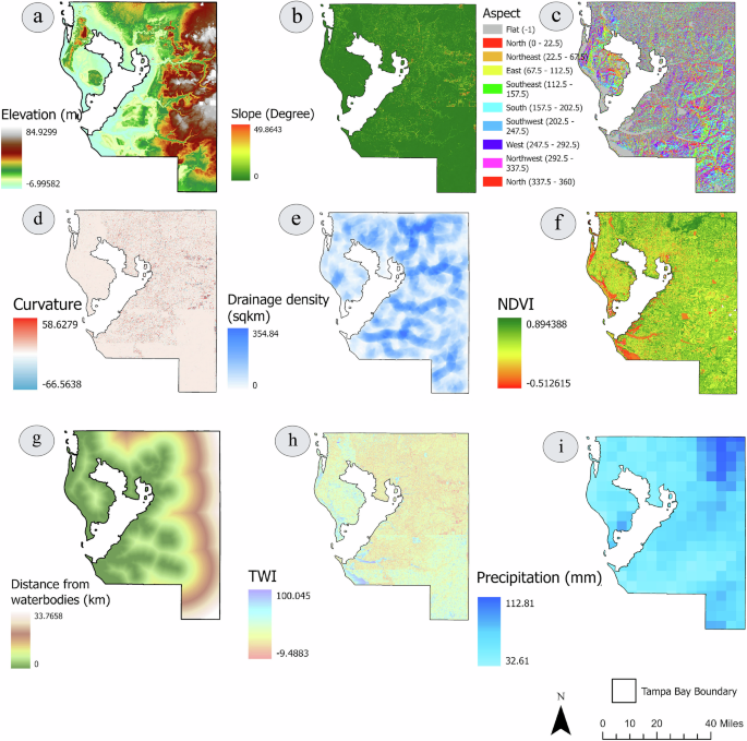
a Elevation; (b) slope; (c) aspect; (d) curvature; (e) drainage density; (f) NDVI; (g) distance from waterbodies; (h) TWI; (i) precipitation. These maps were generated in ArcGIS Pro 2.4.0.
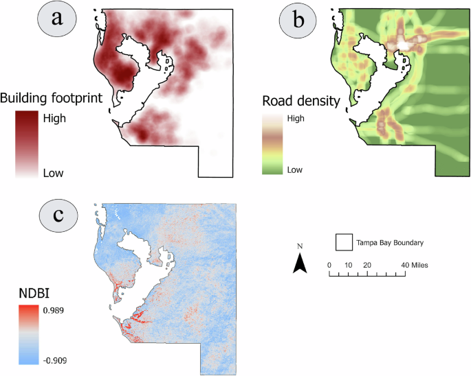
a Building footprint density; (b) road network density; (c) NDBI. These maps were generated in ArcGIS Pro 2.4.0.
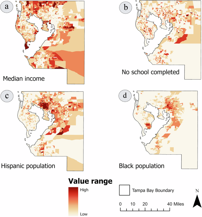
a Median income; (b) percentage of population with no school completion; (c) percentage of Hispanic population; (d) percentage of Black (African American) population. These maps were generated in ArcGIS Pro 2.4.0.
Before selecting these FRFs, this study underwent a multicollinearity analysis to check if any severe correlation exists among them. Conducting a multicollinearity analysis is a crucial step prior to selecting FRFs for flood risk simulation. The value of multicollinearity analysis ranges from −1 to 1. The high correlation between two factors indicates high similarities in data and it has a negative effect on flood risk predictions. So, the factors that have high correlation values above 0.8 and below −0.8 will make predictions inaccurate54. This study thus adopted a threshold value ± 0.8 in selecting FRFs. According to multicollinearity analysis, there is no severe correlation exists among these factors (Fig. 10).
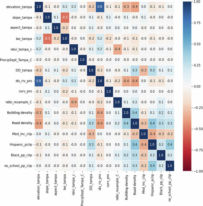
This figure displays the correlation among each FRFs. The X-axis and primary Y-axis represent the name of FRFs. The secondary Y-axis represents the value range of correlation analysis (−1 to +1). Blue color indicates positive correlation and red color indicates negative correlation. The data were processed and plotted in Python 3.11.7.
This study also checked multicollinearity using variance inflation factors (VIF). When VIF is larger than 10, it indicates multicollinearity problem among FRFs55. However, there are no severe correlations among them (Fig. 11). Following that, all these selected FRFs were standardized using the Z-scores equation (Eq. 1) before training and testing the ML models.
where z is the normalized value, x is the value of each data FRF variable, µ is the mean value of the FRF variable, and σ is the standard deviation of the FRF variable.
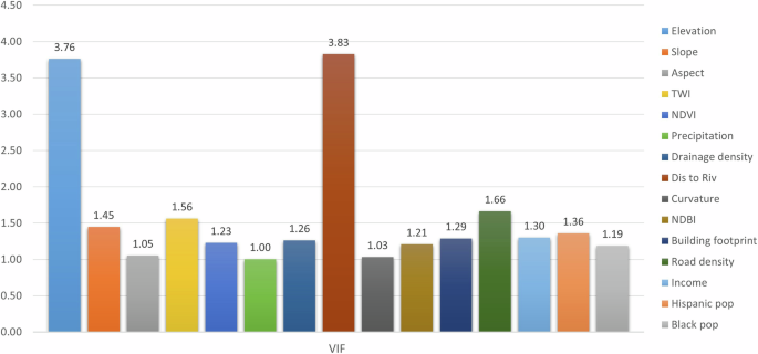
Y-axis represents the range of VIF score. The VIF analysis was conducted in Python 3.11.7.
Machine learning models
This study adopted a total of five ML models including DT, SVM, AdaBoost, XGBoost, and RF. This study employed the default classifier for each ML model to provide an equal basis for evaluation. These models are briefly described below.
Decision tree (DT)
Decision trees algorithm can effectively solve classification, regression, and multi-output problems by fitting complex datasets56. The DT model utilizes hierarchical structure to identify the pattern in data and establish a decision-making rule for estimating the relationship between the independent and dependent variables57. Each DT comprises root nodes, child nodes, and leaf nodes while leaf nodes provide the final prediction. DT models can identify complex relationships between variables and handling both categorical and continuous data without any strict data distribution assumption58. This study used the DT classifier from the SciKit Learn package59.
Support vector machine (SVM)
SVM is a powerful and versatile supervised ML algorithm, able to perform both linear/non-linear classification, and regression. It is also capable of detecting outliers56. It is based on statistical learning theory and the structural risk minimization principle that uses training dataset to map original input space into high dimensional feature space58. Later, an optimal hyperplane is generated by maximizing the margins of class boundaries to separate the points of different classes. The point above the optimal hyperplane is labeled as +1 and the points below the hyperplane are labeled as −160. The closest training points to the optimal hyperplane are known as support vectors. Once the decision boundary is generated, it can be used to classify new data61. This study utilized the SVM classifier from the SciKit Learn package59.
Adaptive boosting (AdaBoost)
Adaptive boosting, commonly known as AdaBoost, is an ensemble ML algorithm that turns a weak learner into a strong learner. A new predictor pays more attention to predecessor training instances that are under-fitted56. This algorithm initially trains a base classifier such as DT by assigning equal weight to all training instances and tries to predict them. Later, this algorithm tries to increase the relative weight of misclassified instances and decrease the weights of correctly classified instances62. After that, this algorithm trains another classifier with updated weights and makes predictions on the training set and updates the instance weights again. This process continues until a perfect predictor is found56. This algorithm provides significant benefits, including solving binary class problems, multi-class single or multi-label problems, and regression problems63. In this study, AdaBoost classifier has been used from the SciKit Learn package59.
Extreme gradient boosting (XGBoost)
Extreme gradient boosting is a scalable ML tree-boosting system proposed by Chen and Guestrin64. It is mainly designed for superior performance and speed. Instead of averaging independent DTs, XGBoost builds a sequence of DTs by targeting prediction errors or residuals from highly uncertain samples generated by previous tree models65. Its numerous tunable parameters and hyperparameter help to increase the predictive accuracy by reducing the overfitting issue and predictive variability66. The XGBoost model was conducted by using XGBclassifier from the xgboost package.
Random forest (RF)
RF, introduced by Breiman67, is a robust ensemble supervised ML algorithm which can solve both classification and regression problems56. This model utilizes bootstrap sampling method to select a subset randomly from training dataset and constructs a DT by recurrently splitting the data based on the best split for each bootstrap sample68. Each DT consists of root, child, and leaf nodes. Leaf nodes provide final prediction through majority voting for classification or mean assessment for regression69. RF models offer several benefits, such as the abilities to identify significant features, to achieve high predictive accuracy, to reduce overfitting, to handle high dimensional data, insensitivity to noise, and to manage missing value70,71. This study utilized the RF classifier from the SciKit Learn package59. The default parameters of these ML models that used in this study are listed in Table 5.
All these five ML models were trained and tested using flood damage points (target variable) and FRFs (predictor variable). The RF and XGBoost were selected based on their slight better performance on ROC–AUC curve and evaluation metrics for further flood risk simulation. To simulate flood risk index (FRI), predict_proba function was used on the RF and XGBoost model. The FRI for each pixel generated from the simulation ranges from 0 to 1, representing the gradual range of flood risk probability. The value close to 0 indicates low flood risk and value close to 1 indicates high flood risk. This study applied equal interval classification method to classify the FRI into five different risk categories including very low (0–0.2), low (0.2–0.4), moderate (0.4–0.6), high (0.6–0.8), and very high (0.8–1.0). Finally, the spatial distribution of flood risk areas across different risk categories was mapped and documented in tables.


Responses