Socially vulnerable communities face disproportionate exposure and susceptibility to U.S. wildfire and prescribed burn smoke

Since the latter part of the 20th century, air pollution from anthropogenic activities in the United States (U.S.) has greatly decreased^1,2,3,4. In contrast, wildfire emissions have risen^{5,6,7,8,9,10,11,12}, particularly in recent years, as highlighted by events in the American West, Canada, Hawaii, and Texas. Fires are sources of ammonia (NH₃), nitrogen oxides (NO_x), primary fine particulate matter (PM_2.5), sulfur dioxide (SO₂), and volatile organic compounds (VOCs)¹³, all of which contribute to concentrations of ambient PM_2.5^14,15,16. Any level of long-term exposure to PM_2.5 is statistically associated with increased mortality risk^17,18. This incremental rise in risk, when combined with estimates of the exposed population size, yields premature mortalities attributable to PM_2.5 exposure¹⁹. This impact area accounts for most health-related damages from air pollution in the U.S.³. Hence, in addition to the costs associated with fires themselves (e.g., flame-related injuries or deaths and property damage), there are substantial costs associated with exposure to the resulting smoke^20,21,22. Moreover, similar pollution risks come from prescribed burns (i.e., controlled fires set intentionally and legally), which are widely employed to mitigate wildfire risks among other purposes^23,24,25,26.

Socially vulnerable populations—namely, people of color (POC) and people of low socioeconomic status—are disproportionally exposed to elevated levels of ambient PM_2.5 in the U.S.^{4,27,28,29,30,31}. For example, average PM_2.5 exposures from all domestic anthropogenic sources in 2014 were 5.9 μg m⁻³ for non-Hispanic or Latino White (White) persons compared to 7.4 μg m⁻³ for POC²⁸. However, disparities pertaining to air pollution are not limited to exposure; inequities also exist in variable susceptibility to pollution. Marginalized populations are more likely to experience chronic illness or other external factors driving elevated distress; such populations are also less likely to have adequate health care^27,32. These factors drive an increased risk from air pollution exposure^33,34. Importantly, senior citizens, another particularly vulnerable subpopulation, also bear more risk from air pollution^35,36 such that they suffer the majority of the associated premature mortality³⁷.

While the field is expanding, the nexus of wildland fire smoke impacts and vulnerability is an understudied topic in the literature. In this study, we focus on smoke exposures and damages as they vary across different levels of vulnerability as defined by the Social Vulnerability Index (SVI)—a census tract-level measure of a community’s ability to adapt to avoid suffering and loss in the event of a disaster^38,39. Our work introduces the AP4T integrated assessment model to investigate the damages caused by ambient PM_2.5 from wildfire smoke (WFS) and prescribed burn smoke (PBS) in census tracts across the contiguous U.S. in 2017. AP4T is an extension of AP4—the newest version of the Air Pollution Emission Experiments and Policy (APEEP) model¹⁶ and its successors, AP2⁴⁰ and AP3⁴¹. AP4T uses emissions data from the National Emissions Inventory (NEI)¹³, a long-term mortality risk dose-response function derived from the American Cancer Society Cancer Prevention Study II¹⁸, and the value of a statistical life (VSL) suggested by the U.S. Environmental Protection Agency (EPA)¹⁹. AP4T evaluates the marginal impacts of emissions from specific sources across more than seventy thousand census tracts, offering a higher resolution than its county-level predecessors, in recognition of the importance of spatial resolution when investigating exposure disparities²⁹. The model also accounts for varying health risks by tract—dictated by age, race/ethnicity, and other geographically variable vulnerability factors—ensuring that inequities associated with pollution are not overlooked by applying a uniform approach³⁷.

This work adds to the growing literature on the air quality burden from fire smoke. Many studies have used state-of-the-science chemical transport models to evaluate downwind air pollution resulting from emissions upwind^{9,10,12,42,43,44}, but these tools require substantial time, resources, and expertise to operate⁴⁵. Other work has employed satellite imagery and ground monitor data along with statistical modeling, observable concentration spikes, or air parcel trajectory assessments to isolate smoke pollution from background levels^{5,6,7,8,11,46}. With imaging- and monitoring-related methods, however, source attribution (i.e., linking impacts to their origin) remains difficult, and evidence suggests that PBS is more difficult for imaging- and monitoring-related methods to identify²⁶. AP4T’s reduced-complexity air quality modeling (RCM) framework offers a more computationally efficient alternative to chemical transport models while delivering comparable results in terms of predicted ambient PM_2.5⁴⁵. It also enables a direct linkage between highly granular sources and receptors across a wide range of simulated scenarios.

Many studies have found that fire smoke, like other air pollutants, is associated with increased morbidity and mortality risk^{11,20,26,47,48,49,50}. Until recently, however, the associated social costs were less well understood^20,51. While largely dependent on the fires assessed and other study-specific factors, research suggests that damages are on the order of billions of dollars^10,44,49,52. As previously noted, the intersection of fire smoke impacts and vulnerability remains a relatively unexplored area in the literature. Some studies have shown that smoke exposure correlates positively with vulnerability indicators that are known to exacerbate risk^43,44,53,54, while others have found that, contrary to other emission sources²⁸, exposure to fire smoke increases with income and as the percentage of White people within a population rises^5,6. We contribute to this growing body of knowledge by calculating social costs for populations differentiated by various demographic attributes and analyzing the drivers of the results across identifiable components of the AP4T integrated assessment model (i.e., exposure, susceptibility, and valuation) and the SVI (e.g., race/ethnicity, socioeconomic status, and age). Our work provides essential insights for decision-makers addressing the increasing environmental hazard of fire smoke, particularly its impact on vulnerable communities. More broadly, it contributes to the ongoing conversation around environmental justice related to air pollution, a topic made especially complex by the intricate relationships among different aspects of social vulnerability.

Our primary findings are as follows. Damages from fire smoke in 2017 amounted to more than $200 billion (17% of the total across all emission sources in the contiguous U.S.). The monetary damages are from approximately 20 thousand premature deaths; roughly half were due to WFS, and half were due to PBS. WFS is mostly produced in and received by California and the western U.S., while PBS affects a broader geographic area of the southeastern U.S. There is a positive correlation between social vulnerability and WFS exposure. This is also true for PBS and above-average vulnerability, but the association is less prominent. These observations hold in some regions (and states) but are primarily driven by between-state rather than within-state relationships of smoke and vulnerability. When incorporating susceptibility into the analysis, observed trends change markedly due to the relationships between age and social vulnerability (negatively correlated for most criteria) and age and PM_2.5 health risks (positively correlated). While senior citizens (65 and older) accounted for 16% of the population, they suffered 75% of the damages from 2017 fire smoke. Of further note is the relationship between age and race/ethnicity in the U.S. Because POC is younger than White people on average, POC (who tend to be more vulnerable than White people) experience less damage per capita overall. However, POC incur more damage per capita within age groups. Our work reveals the immense social costs from wildland fire smoke, offers tools for identifying particularly damaging sources and damaged receptors, highlights the age-race/ethnicity-social vulnerability nexus and the resulting implications for air pollution impacts, and informs decision-makers seeking to address this escalating environmental hazard.

Sources and receptors of damages from wildfire and prescribed burn emissions

In 2017, national air quality damages from wildland fire smoke were $201 billion (or 20.1 thousand premature deaths). This amounts to 17% of the total damages from all emissions modeled by AP4T ($1.20 trillion, 121 thousand deaths). Of the total fire smoke damages, half were from WFS ($99.4 billion or 8.3% of all sources), and half were from PBS ($101 billion or 8.4% of all sources). See the Methods section for a sensitivity analysis on damages using alternative modeling inputs. Figure 1a shows 2017 air pollution damages from WFS (top) and PBS (bottom) by location of emissions (left) and the resulting smoke (right). Spatial variability in damages is a function of multiple factors: (1) where and what the fires burn, (2) how the emissions transport downwind and behave chemically in the atmosphere, (3) where populations are located relative to smoke dispersion, and (4) how susceptible the exposed populations are to PM_2.5 pollution.

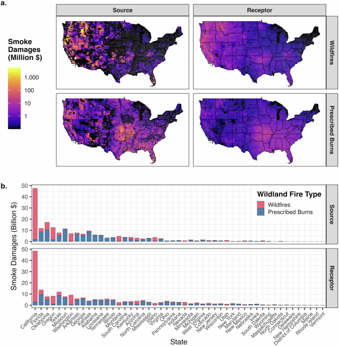
a Smoke damage mapped at the census tract level. The color scale is log-transformed. b Smoke damages totaled at the state level. States are ordered from left to right by most-to-least total wildland fire smoke damages, averaged between those by source location and those by receptor location. a, b Data characterize 2017. Damages are in 2020 U.S. dollars. Wildfire smoke damages are out of $99.4 billion in total. Prescribed burn smoke damages are out of $101 billion total. Sources are where and from what emissions are generated. Receptors are where pollution is experienced. See Supplementary Fig. 22 for smoke PM_2.5 by census tract from wildfires and prescribed burns. See Supplementary Note 1 for additional analysis and discussion of state-level fire smoke damages. Mapping uses the rgdal R package¹¹⁷. Plotting uses the ggplot2 R package¹¹⁸.

Full size image

There is a clear difference between where wildfires and prescribed burns predominantly occur. The EPA’s NEI reports that in 2017, most wildfire emissions in the contiguous U.S. came from the western states¹³ (see Supplementary Table 1 for wildfire and prescribed burn emissions by state). To illustrate, 75% of primary PM_2.5 emissions from wildfires were released from just five states: California, Oregon, Montana, Idaho, and Washington. On the other hand, most emissions from prescribed burns were released from states throughout the southeastern U.S. For example, 59% of primary PM_2.5 emissions were from the following seven states: Oklahoma, Kansas, Missouri, Florida, Arkansas, Texas, and Louisiana. For both WFS and PBS, relative state contributions were similar for NH₃, NO_x, SO₂, and VOCs, but primary PM_2.5 accounts for more than 70% of the air pollution damages from fire emissions (see Supplementary Table 2). For total emissions of NH₃, NO_x, primary PM_2.5, SO₂, and VOCs from wildfires and prescribed burns compared to national totals from all sources, see Supplementary Table 3.

Importantly, there is heterogeneity in damages per tonne, driven by discharge location, which explains how wildfires can emit more pollution but result in fewer damages than prescribed burns (see Supplementary Table 2). Atmospheric processes carry pollution across state lines and, often, across regions. We connect spatially resolved emissions through air quality modeling (pollutant dispersion and chemistry) to spatially resolved concentration estimates. Specifically, AP4T employs a Gaussian plume-based RCM⁵⁵ to estimate the PM_2.5 concentrations in every census tract resulting from emissions from a particular source. It then runs location-specific health impact modules—using population⁵⁶, mortality rate⁵⁷, and concentration-response^18,58 data—to estimate premature deaths from PM_2.5 exposure. AP4T then applies a uniform VSL, at $9.97 million per capita, to monetize mortality risk^19,59,60. The spatial structure of AP4T produces a matrix of damages that depicts how emissions from a particular location cause damages in each downwind receptor at the tract level. Aggregating all receptor damages attributable to each emission source produces the left-side maps of Fig. 1a. For each receptor, adding up damages from all sources yields the right-side maps.

Figure 1b shows damages produced (top) and received (bottom) by every state in the contiguous U.S. Aligning with similar work¹¹, we find that California was the greatest source and recipient of WFS damages by far (46% for both), driven by substantial wildfire activity (25% of wildfire emissions¹³) but also its large population (12% of the contiguous U.S.⁵⁶). California, Oregon, Washington, Oklahoma, Montana, and Idaho—the six states contributing the most WFS damages—account for 78% of damages by origin and 68% of damages by destination. No one state dominated for PBS damages to the degree that California did for WFS damages. Missouri, Oklahoma, Florida, Kansas, Arkansas, and Texas accounted for 51% of damages by origin and 38% of damages by destination; adding Georgia, Alabama, Louisiana, and South Carolina add 20% and 17%, respectively. See Supplementary Note 1 and Supplementary Tables 4–6 for additional analysis and discussion of region-, state-, and county-level fire smoke damages.

We also examine fire event-specific damages in Supplementary Note 2, Supplementary Fig. 1, and Supplementary Tables 7 and 8. For example, in addition to destroying more than five thousand structures and killing 22 people, the Tubbs wildfire in Napa and Sonoma counties—the second most destructive in California’s history and the second deadliest of the 21st century, surpassed only by the 2018 Camp Fire—caused $2.47 billion in WFS damages (248 premature deaths)²². This fire was one of several that ignited in the North Bay Area in early October under severe fire weather conditions, collectively causing over $6 billion in physical damages²². The smoke from these fires caused nearly $8 billion in damages (797 premature deaths), highlighting that the social costs of fire emissions can rival the physical costs of even the most devastating wildfires.

Fire smoke exposure by social vulnerability

Population is a primary driver of social costs from air pollution: generally, the more people are exposed, the more damage. Population heavily influences the distribution of damages by county (see, for example, Supplementary Table 6)—the resolution of AP4T’s parent model, AP4, and its predecessors. AP4T’s tract-level resolution reduces the influence of population counts on received damages across space since tracts are explicitly designed to cover approximately equal numbers of people. However, there is still variability by tract (see Supplementary Table 9). Hence, we use population-weighted average exposures and damages per capita in our impact distribution assessments.

The SVI, derived from 15 social vulnerability variables (detailed in the Methods section), provides summary data to help planners and responders identify locations that may need the most support in the event of a disaster^38,39. For our analyses, we divide tracts into SVI deciles, ranging from 1 (10% least vulnerable tracts) to 10 (10% most vulnerable tracts). The bars in Fig. 2a show percentage differences in average exposures for each SVI decile relative to the national average for each fire type: 0.708 μg m⁻³ for WFS and 0.625 μg m⁻³ for PBS. We find that WFS exposure and the SVI are positively correlated; exposure increases as the deciles increase from 1 to 10. WFS exposures for the four least vulnerable deciles of tracts are statistically significantly lower than the national average, while those for the four most vulnerable deciles of tracts are statistically significantly higher. We see weaker evidence of a positive correlation between PBS exposure and SVI status. However, SVI deciles 1–3 are exposed less and SVI deciles 6 to 9 are exposed more, all to extents that are statistically significant. See Supplementary Tables 10 and 11 for statistical significance indicators of average exposure differences derived using t-tests.

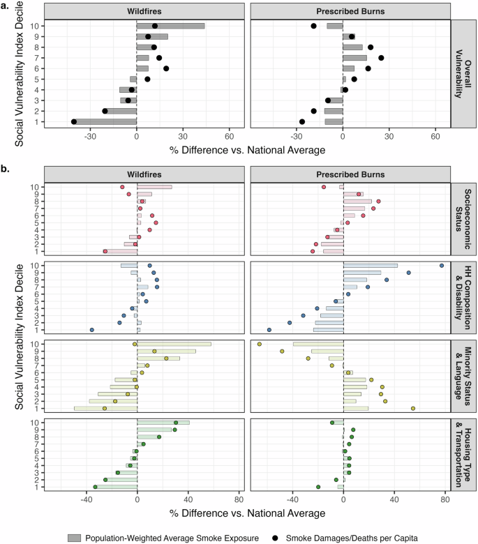
a Smoke impact disparities by overall Social Vulnerability Index decile. b Impact disparities by themed Social Vulnerability Index decile: Socioeconomic Status (Theme 1, red), HH (Household) Composition & Disability (Theme 2, blue), Minority Status & Language (Theme 3, yellow), and Housing Type & Transportation (Theme 4, green). a, b Data characterize 2017. Tracts are divided into deciles from least (1) to most (10) vulnerable using Social Vulnerability Index percentile ranks^38,39. Observations are percentage differences from the national average: 0.708 μg m⁻³ and $308 per person for wildfire smoke and 0.625 μg m⁻³ and $313 per person for prescribed burn smoke. See Supplementary Tables 10 and 11 for statistical significance indicators of impact differences derived using t-tests. Plotting uses the ggplot2 R package¹¹⁸.

Full size image

The bars in Fig. 2b show exposure disparities across different levels of vulnerability for each of the SVI’s four themes: Socioeconomic Status (Theme 1), Household Composition & Disability (Theme 2), Minority Status & Language (Theme 3), and Housing Type & Transportation (Theme 4). For this analysis, we define SVI deciles distinctly for each individual theme. The positive correlation between WFS and overall vulnerability manifests for SVI themes 1, 3, and 4. For PBS, Theme 3 shows a clear negative trend with smoke exposure, while Theme 2 shows a clear positive trend.

We further investigate the exposure disparities observed in Fig. 2 by evaluating regions (Fig. 3) and states (Fig. 4). Figure 3a shows smoke exposure by overall SVI decile within the nine census divisions (see Supplementary Figs. 2 and 3 for themed SVI iterations). SVI deciles are not redesignated within divisions. We see that, for WFS, the positive correlation at the national level is only clearly evident for the highly WFS-exposed Pacific division (i.e., California, Oregon, and Washington). Importantly, stark positive correlations between PBS and the SVI are evident within the four most PBS-exposed census divisions, but the most vulnerable tracts (SVI decile 10) are the least exposed in two of these divisions. Figure 3b helps explain the exposure disparities at the national level (see Supplementary Fig. 4 for themed SVI iterations). Despite within-division disparities, populations in the West and the South generally experience higher exposures to WFS and PBS, respectively. It is the distribution of social vulnerability that drives national trends—some of the most smoke-exposed regions host a disproportionate percentage of the most vulnerable people in the U.S. This results in the higher SVI deciles receiving more weight from these highly exposed regions. In contrast, the Northeast (particularly, New England) is home to higher percentages of less vulnerable people, resulting in the opposite effect.

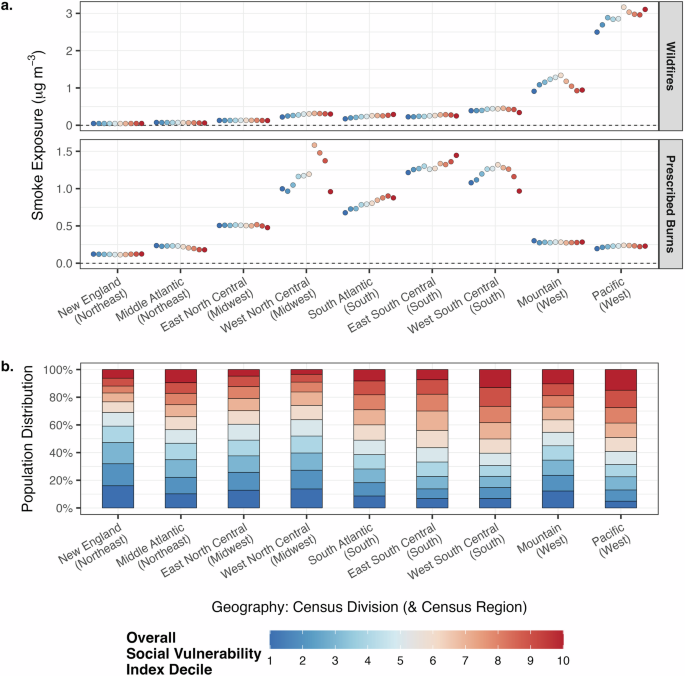
a Population-weighted average smoke exposure (μg m⁻³) by overall Social Vulnerability Index decile within census divisions. b Percentage of census divisions’ populations⁵⁶ in each Social Vulnerability Index decile. An equal distribution of vulnerability across the contiguous U.S. would result in each decile accounting for 10% of every census division’s population. a, b Data characterize 2017. Tracts are divided into deciles from least (1) to most (10) vulnerable using Social Vulnerability Index percentile ranks^38,39. Red represents more vulnerable (from 10 down), and blue represents less vulnerable (from 1 up). See Supplementary Note 1 for the states included in each census division. Census regions are in parentheses after census divisions. See Supplementary Figs. 2–4 for themed Social Vulnerability Index iterations. See Supplementary Table 4 for smoke damages by census division and region. Plotting uses the ggplot2 R package¹¹⁸.

Full size image

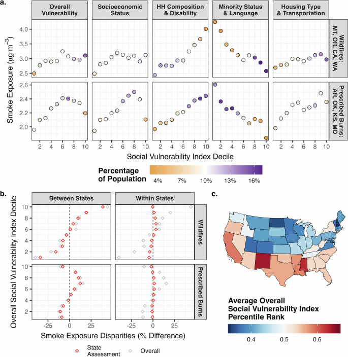
a Population-weighted average smoke exposure (μg m⁻³) by overall and themed Social Vulnerability Index decile within the four most smoke-polluted states for each fire type: MT (Montana), OR (Oregon), CA (California), and WA (Washington) for wildfires and AR (Arkansas), OK (Oklahoma), KS (Kansas), and MO (Missouri) for prescribed burns. Color scale represents the percentage of the states’ populations⁵⁶ accounted for by each decile. White represents 10% of states’ populations, an equitable representation of the decile. Purple represents >10%, an over-representation of the decile. Orange represents <10%, an under-representation of the decile. b Between- and within-state disparities by overall Social Vulnerability Index decile. Between-state analysis assigns each person their state’s population-weighted average smoke exposure. The within-state analysis compares each person’s tract-level smoke exposure to their state’s population-weighted average smoke exposure. c Average overall Social Vulnerability Index percentile rank by state. a–c Data characterize 2017. Tracts are divided into deciles from least (1) to most (10) vulnerable using Social Vulnerability Index percentile ranks^38,39. See Supplementary Figs. 5 and 6 for impact versus vulnerability assessments in the ten most smoke-polluted states and Supplementary Figs. 7–9 for themed SVI iterations corresponding to (b) and (c). Mapping uses the usmap R package¹¹⁹. Plotting uses the ggplot2 R package¹¹⁸.

Full size image

Figure 4a presents smoke exposure by overall and themed SVI decile within the four most smoke-polluted states by fire type. SVI deciles are not redesignated within states. Montana, Oregon, California, and Washington residents were exposed most to WFS (all >2.7 μg m⁻³), and Arkansas, Oklahoma, Kansas, and Missouri residents were exposed most to PBS (all >2.0 μg m⁻³). The color scale in Fig. 4a shows the percentage of the states’ populations accounted for by each SVI decile; 10% (white) indicates that the states host an equitable share of the SVI decile, while more (purple) and less (orange) than 10% signify over- and under-representations, respectively.

Comparing Fig. 4a to Fig. 2 reinforces the hypothesis that population distributions drive national trends. This is especially clear with Themes 2 and 3 for WFS exposures. In the most exposed states, Household Composition & Disability vulnerability shows a positive correlation with WFS, while Minority Status & Language vulnerability shows a negative correlation—patterns that contrast with those observed across the contiguous U.S. The divergence stems from between-state vulnerability and smoke exposure trends, as emphasized in Fig. 4b. This analysis compares state-level smoke exposures to the national average (between-state) and tract-level smoke exposures to state averages (within-state). Finally, Fig. 4c demonstrates how the distribution of social vulnerability across states influences the observed correlations with smoke exposure. See Supplementary Figs. 5 and 6 for impact versus vulnerability assessments in the ten most smoke-polluted states and Supplementary Figs. 7–9 for themed SVI iterations corresponding to Fig. 4b, c.

Fire smoke damages by social vulnerability

Normalizing by population makes damages a function of two variables: exposure and susceptibility since the VSL is applied uniformly at $9.97 million. The points in Fig. 2a show percentage differences in damages per capita for each SVI decile relative to the national average for each fire type: $308 per person for WFS and $313 per person for PBS. Interestingly, the literature suggests that all else equal, susceptibility to exposure would be greater for more vulnerable populations^27,32,33,34, but this is not what Fig. 2a reveals. Compared to smoke exposure, relative impacts increase for populations identified as being at approximately the median of the SVI and decrease for both the least and most vulnerable populations.

The points in Fig. 2b reflect damages per capita by SVI theme. We see that, in terms of relative impacts, damages increase substantially from exposures for the most vulnerable individuals under Theme 2 (Household Composition & Disability). Contrarily, relative damages decrease substantially from relative exposures for the most vulnerable individuals under Theme 3 (Minority Status & Language). We also see that Themes 2 and 3 experience the opposite trends in relative impact differences for the least vulnerable people. Relative impact differences for Theme 1 (Socioeconomic Status) and Theme 4 (Housing Type & Transportation) exhibit more similarity to the trends observed for Theme 3—i.e., relative impacts for the most vulnerable decrease from exposures to damages—rather than those observed for Theme 2, but there is more ambiguity.

Figure 5 takes a deeper look at the SVI with analyses considering its 15 social vulnerability variables. Both plots show the fitted coefficients from bivariate linear models (see Supplementary Methods 4) that regress natural log-transformed smoke exposure (Fig. 5a) and damages per capita (Fig. 5b) on social vulnerability variable percentile ranks^38,39 (see Supplementary Table 12 for statistical significance indicators based on p-values). Figure 5a shows that three variables exhibit the strongest positive relationships with WFS exposure: the percentage of people who are non-White, the percentage of people who speak English “less than well,” and the percentage of households characterized by crowding, all variables that exhibit negative relationships with PBS exposure. This is driven by the overrepresentation of these social vulnerability variables in the West (see Supplementary Table 13), particularly in California (see Supplementary Fig. 10), where PBS levels are low. The greatest PBS coefficients correspond to the percentage of civilians with a disability and the percentage of households that are mobile homes, followed closely by per capita income and the percentage of people below the poverty line. Notably, WFS and PBS both have negative relationships with the percentage of households with no vehicle access, a vulnerability trait most prevalent in the Northeast.

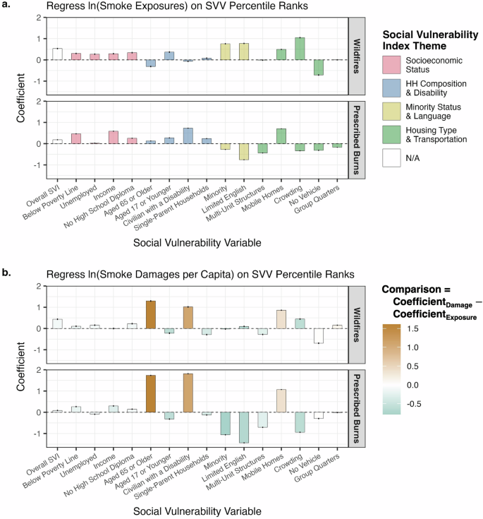
a Coefficients from unique bivariate linear regressions of natural log-transformed smoke exposure on social vulnerability variable (SVV) percentile ranks at the tract level. Colors represent the social vulnerability variables’ respective themes. b Coefficients from unique bivariate linear regressions of natural log-transformed damages per capita on social vulnerability variable percentile ranks at the tract level. White represents equal damage and exposure coefficients. Green represents a lower damage coefficient than exposure coefficient. Brown represents a higher damage coefficient than exposure coefficient. a, b Data characterize 2017. Coefficients are the percentage changes in impacts per 0.01 increase in the social vulnerability variable percentile ranks, which range from 0 to 1. Error bars show 95% confidence intervals derived using bootstrapping. Social vulnerability variables are those comprising the Social Vulnerability Index (SVI)^38,39. See Supplementary Methods 4 for details on the regression modeling and statistical analysis. See Supplementary Table 12 for coefficients, 95% confidence intervals, statistical significance indicators, and comparisons guiding the color scale in (b). Plotting uses the ggplot2 R package¹¹⁸.

Full size image

Moving from Fig. 5a to Fig. 5b supports the observations from Fig. 2. The color scale in Fig. 5b shows the difference between coefficients for damages per capita and coefficients for exposures. Green shows where susceptibility—which has an influence on damages per capita but not exposures—lowers the association between smoke impacts and each vulnerability variable, and brown shows the opposite. The increase in coefficients from exposures to damages is by far the greatest for the percentage of people 65 and older and the percentage of civilians with a disability, two variables within Theme 2. On the other hand, many of the social vulnerability variables see a decrease in coefficients from exposures to damages. This change is most substantial for the percentage of people 17 and younger as well as other variables that are highly correlated with younger people (see Supplementary Table 14). The following section explores an occurrence of Simpson’s Paradox—where trends within groups differ from the overall trend due to the presence of a confounding variable. Here, the confounding variable is age, a critical factor that influences both air pollution damages and social vulnerability.

Fire smoke damages per capita by race/ethnicity and age group

The relationships between age and different vulnerability variables explain important aspects of the difference between exposure and damage disparities along the SVI scale (see Supplementary Tables 14–18 for relevant correlations). This is well-illustrated by looking at how fire smoke damages per capita vary by race/ethnicity and age group subpopulations. Age is a key factor that dictates susceptibility to PM_2.5 exposure. Baseline mortality risk, which increases exponentially with age⁵⁷ (see Supplementary Table 19), is a multiplicative input to the mortality concentration-response function¹⁸ (see Eq. 4 of the Methods section).

An important point is that POC populations are younger than the White population in the U.S. Figure 6a breaks down each race/ethnicity, as identified by the U.S. Census Bureau⁵⁶, into age intervals for 2017. The pie charts show that White is the only subgroup with people under 40 accounting for less than half of the total population and people over 60 accounting for more than a quarter of the total population. Americans who are 80 and older make up 4.8% of the White population but no more than 2.5% of any other subgroup. See Supplementary Fig. 11 for pie charts showing the opposite breakdown—age groups by race/ethnicity.

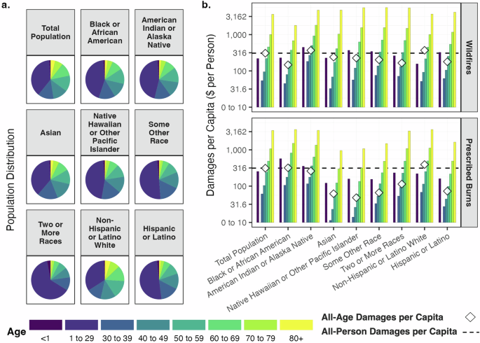
a Population breakdown by age group for each race/ethnicity. Subpopulation breakdowns consider totals across the contiguous U.S⁵⁶. Pie charts represent youngest to oldest age group, reading counterclockwise from the top. b Damages per capita overall and by age group for each race/ethnicity. Damages are in 2020 U.S. dollars. y-axes are log-transformed and include breaks from 0 to 10 $ per person. Ages 1–29 experience no damage^18,58. Dashed black lines represent damages per capita across all populations: $308 per person for wildfire smoke and $313 per person for prescribed burn smoke. White diamonds represent damages per capita across all populations within each race/ethnicity subgroup. Baseline risk (mortality rates) are differentiated by race/ethnicity. Relative risk is not differentiated by race/ethnicity. a, b Data characterize 2017. Subpopulations other than non-Hispanic or Latino White are not mutually exclusive. All racial subgroups except non-Hispanic or Latino White include persons of Hispanic or Latino ethnicity. Hispanic or Latino ethnicity includes persons of all racial subgroups except White. See Supplementary Tables 22 and 23 for fire smoke damages per capita by race/ethnicity and age and disparities within age groups, respectively. Plotting uses the ggplot2 R package¹¹⁸.

Full size image

Figure 6b reveals the substantial influence of age (through baseline mortality risk) on damages per capita (note: the vertical axis in Fig. 6b is log-transformed). As noted previously, national damages per capita were $308 and $313 for WFS and PBS in 2017, respectively (shown by the black dashed lines in Fig. 6b). Critically, our default concentration-response modeling is based on epidemiological studies that find statistically significant evidence of premature mortality risk from PM_2.5 for infants⁵⁸ and populations 30 years and older¹⁸ (see Supplementary Table 20). Hence, no damages are incurred within the 1–29 age group. For people over 30, there are large increases in damages per capita by ten-year age groups. People in their thirties, forties, fifties, sixties, and seventies incurred total fire smoke (WFS plus PBS) damages of $115, $199, $463, $947, and $2070 per capita. Damages per capita for 80 years and older were $7040.

Figure 6b shows that the influence of age holds within each race/ethnicity. While there is variation in damages per capita by race/ethnicity (shown by the white diamonds in Fig. 6b), variation by age within each group is far more substantial. We see that, overall, only American Indian or Alaska Native (Native American) and White persons incurred more damage from WFS than average. This was driven by above-average exposures for Native American persons, who were exposed to 67% higher levels of WFS than the average person (see Supplementary Fig. 12 for WFS and PBS exposures by race/ethnicity), and greater age-adjusted baseline health risks (see Supplementary Table 21 for mortality rate disparities by race/ethnicity within age groups). Notably, this exposure disparity can be explained by the fact that a large proportion of Native American individuals reside in the West (see Supplementary Fig. 13). In contrast, White persons were exposed to 12% lower levels of WFS than average and, for the most part, experienced average age-adjusted baseline health risks. It was neither exposure nor age-adjusted susceptibility that resulted in above-average WFS damages per capita for White persons. Rather, the age distribution for the White population was older. This point is further supported by the fact that damages per capita for Hispanic or Latino persons (as well as for several other race/ethnicity subpopulations) were greater than those for White persons within every age group. However, the much younger Hispanic or Latino population has far lower than average damages per capita overall.

For PBS, both Black or African American (Black) individuals and White individuals experienced greater damage than average. Black persons (a large proportion of whom reside in the Southeast, as shown in Supplementary Fig. 13) experienced 22% higher exposure to PBS than average, while White persons incurred only 4.8% higher exposure than average. Additionally, in contrast to White persons, Black persons also experienced greater age-adjusted baseline health risks. Within age groups, White persons suffered damages no more than 12% greater than average. Overall, White persons suffered damages 25% greater than average. For Black persons, damages were no less than 22% greater than average within every age group (except the oldest), but all-age damages were only 2.0% greater than average. See Supplementary Tables 22 and 23 for fire smoke damages per capita by race/ethnicity and age and disparities within age groups, respectively.

These asymmetries between overall and age-adjusted damage disparities manifest because older Americans are overwhelmingly White, as shown in Fig. 6a. Per capita damages incurred by senior citizens pull White damages per capita upward while pushing POC damages per capita downward. It is not that White persons experienced more damage ceteris paribus; it is that older people heavily influence the average damage across all age groups. While only accounting for 16% of the U.S. population, senior citizens suffered 75% of fire smoke damages. Moreover, 31% of damages occurred within the 85 and older age group, which comprised less than 2% of the population. The total population was 61% White, the senior citizen population was 73% White, and the 85 and older population was 78% White. White senior citizens (11% of Americans) and White people over 85 (1.6% of Americans) suffered 58% and 25% of total wildland fire smoke damages, respectively.

Wildfire activity is increasing^{5,6,7,8,9,10,11,12}, and our results suggest wildland fire smoke drives extraordinary costs—over $200 billion in air pollution damages in 2017, 17% of the national total. Nearly half of these were from wildfires, mostly occurring in California and other states in the West. The rest were from prescribed burns, which were regionally concentrated in the Southeast. Marginalized populations are exposed to more pollution from most emission sources in the U.S.^{4,27,28,29,30,31}. Accordingly, we find a positive correlation between smoke exposure and social vulnerability, particularly clear for WFS but still evident for PBS. This is primarily driven by regional trends in both smoke and the SVI—the West and Southeast account for disproportionate shares of the most vulnerable populations in the U.S. That said, positive associations also manifest in some of the most smoke-polluted regions.

Modeling health effects, rather than just exposures, complicates the correlation between impacts and social vulnerability due to the heavy influence of age. In 2017, senior citizens accounted for just 16% of the population but experienced 75% of smoke damages. Besides senior citizenship, however, drivers of vulnerability—namely POC status—are more prevalent among younger people (see Supplementary Tables 14–18 for correlations between vulnerability, age, and race/ethnicity). We find that damages per capita are greater than average for Native American persons from WFS, Black persons from PBS, and White persons from all fire smoke. Increased exposures and baseline risks within age groups drive these results for Native American and Black persons. Contrarily, a greater baseline risk overall due to a larger senior citizen population drives these results for White persons.

While our primary focus is on smoke damages, it is important to acknowledge broader impacts. Wildfires are destructive and deadly, posing severe risks to human lives, property, and ecosystems^20,21,22. In contrast, prescribed burns offer substantial benefits, particularly in reducing wildfire risks by decreasing their likelihood and intensity^23,24,26, which ultimately helps protect nearby communities despite the initial pollution they cause. Moreover, prescribed burns are a land management tool used to maintain and restore healthy ecosystems^{26,61,62,63,64}, and they emit fewer pollutants per acre burned compared to wildfires^25,65,66.

Our research indicates that both the West and Southeast experienced substantial fire smoke damage in 2017. However, while the West bears the additional costs associated with wildfires, the Southeast benefits from the other advantages of prescribed burns. Geographic differences in prescribed burn activities across the U.S. are shaped by a mix of historical factors^63,64, sociopolitical landscapes^67,68,69, and environmental conditions^70,71, leading to 80% of all prescribed burns occurring in the Southeast⁶⁷. In contrast, the West faces numerous barriers to controlled burns⁷⁰, hindering their expansion despite growing calls for increased implementation^67,70,72,73. Notably, these barriers include stricter liability laws and local air quality regulations⁷⁰, which are often designed to protect vulnerable populations. This creates a complex decision-making landscape for prescribed burns. Although they are carefully planned to minimize pollution in nearby communities²⁵, these burns still cause smoke damage, representing a trade-off to mitigate wildfire risks. Therefore, further research into the full range of benefits and costs of prescribed burns, versus the alternative of forgoing them, is essential for identifying the most effective strategies to protect vulnerable populations in a broader context.

Regardless of whether future emissions originate from wildfires or prescribed burns, policymakers have a unique opportunity to address this source of air pollution, as smoke events are episodic. A multipronged approach could provide substantial benefits to communities most at risk²⁴. First, expanding real-time air quality monitoring and enhancing public outreach—particularly through trusted community leaders—in smoke-prone areas could better inform vulnerable and historically marginalized groups on how to adapt. Second, because indoor air quality also deteriorates during smoke events^21,46, investing in filtration technologies^74,75 could establish clean air spaces in locations strategically targeted at vulnerable populations and accessible to the public, such as senior centers in lower-income neighborhoods. A complementary strategy could involve distributing respiratory protection, such as N95 masks⁷⁶, through well-coordinated systems before or during smoke events to safeguard populations with limited access to safe indoor spaces, including outdoor workers^21,24. Ultimately, these solutions depend on robust wildfire emergency response planning⁷⁷ and enhanced decision-making frameworks—including impact forecasting tools^78,79—for prescribed burns. Further research is needed to assess how these measures could mitigate damages and better inform regulators about the net benefits of implementing these solutions.

This analysis indicates that decision-makers should prioritize managing fire smoke risks for senior citizens while also recognizing that assessing PM_2.5 health damages without considering the intersection of vulnerability—particularly race/ethnicity—and age may yield misleading conclusions. It is crucial to acknowledge that disparities within age groups vary based on different vulnerability metrics, especially given the historical factors that have shaped U.S. population demographics. While fire smoke damages are concentrated in White communities, largely due to the high proportion of White senior citizens, this perspective overlooks the impact of disparate hazards (including, but not limited to, air pollution) that reduce the likelihood for the most vulnerable populations—particularly Black and Native American individuals—to reach senior citizenship and the higher PM_2.5 risks. Adopting a more holistic environmental justice perspective is essential.

Several caveats regarding air quality and health effects modeling, discussed in the Methods section, should be considered when interpreting our findings. Most notable are the changes in our results when using alternative modeling approaches that shift the distributional impacts of smoke damages. Specifically, accounting for relative risk differences by race/ethnicity³³ and applying the value of a statistical life year (VSLY) approach^80,81 attribute a greater share of damages to younger, more vulnerable POC. For sensitivity analyses that quantify the uncertainty associated with our results, see the Methods section.

Despite these complexities, the core message remains clear and robust: fire smoke poses substantial risks to both vulnerable and broader populations in the U.S. This work provides a roadmap for identifying communities most in need of attention, including senior citizens, Native American communities in the West, and Black communities in the Southeast. Our research can help guide national, state, and local planners to understand the sources and receptors of damage and identify the populations that would benefit most from efforts to mitigate the impacts of wildland fire smoke.

Reduced-complexity air quality modeling in AP4T

We model wildland fire smoke using 2017 emissions of NH₃, NO_x, primary PM_2.5, SO₂, and VOCs from wildfires and prescribed burns, reported at the county level by the EPA’s NEI¹³. The NEI employs a multi-step approach to estimate emissions from fires, beginning with the collection of fire activity data from state, local, tribal, and national organizations. This data is then supplemented by geographic information system-based analysis and fuel consumption modeling to calculate the resulting emissions. Wildfire and prescribed burn emissions across the contiguous U.S. in 2017 are reported in Supplementary Table 2. Importantly, our study does not include emissions associated with agricultural or pile burning, which are specific types of controlled burns.

For this research, we focus exclusively on 2017, though fire activity fluctuates from year to year^5,12. Our decision to focus on 2017 is partly to maintain simplicity, avoiding the introduction of additional complexity, but also because the AP4T model incorporates several 2017-specific inputs, which are discussed in later sections. Nevertheless, we find that 2017 serves as a reasonable representation of typical fire emissions, as evidenced by Supplementary Figs. 14–16 and Supplementary Tables 24 and 25, which compare 2017 data with that of 2014 and 2020. However, emissions from wildfires grew markedly from 2014 to 2017 (88% increase in primary PM_2.5) and again from 2017 to 2020 (20% increase in primary PM_2.5). For a further discussion, see Supplementary Note 3. Furthermore, there are large uncertainties associated with emission estimates from fires. To better understand and quantify this uncertainty, we compare the NEI with an alternative inventory, the Global Fire Emissions Database (GFED)^82,83. Generally, the GFED reports fewer emissions from fires than the NEI. Further analysis and discussion can be found in Supplementary Note 4 and Supplementary Figs. 17–19.

This paper introduces the AP4T model, an extension of AP4—the newest version of the APEEP model series^16,40,41. AP4T expands the RCM capabilities of AP4 to consider the marginal impacts of emissions at the census tract level. These tools model baseline ambient PM_2.5 resulting from all annual emissions of NH₃, NO_x, primary PM_2.5, SO₂, and VOCs from all sources throughout the contiguous U.S., provided by the EPA’s 2017 NEI¹³. The model employs Gaussian plume-based pollutant transport⁵⁵ to estimate speciated concentrations downwind. A supplemental chemistry module accounts for interpollutant chemistry to determine total PM_2.5, a combination of directly emitted PM_2.5, organic aerosols, ammonium, sulfates, and nitrates. AP4T’s predictions of PM_2.5 are calibrated using the EPA’s Air Quality System monitor data⁸⁴.

The receptors in AP4 (i.e., where damages are experienced) are defined at the county level, as in previous versions of the model. AP4T downscales these receptors. Equation 1 shows the source-receptor (({rm{SR}})) framework, which models the transport ((t)) of a ton of pollution from each source ((s)) to each receptor ((r)) by pollutant ((p)) and bin height ((h)). Atmospheric dispersion behaves differently based on the height of pollutant discharge, so the model divides emission sources into bins that treat ground-level sources differently than point sources and divides point sources into electric generating units (EGUs) and non-EGUs. The point of release at facilities is modeled considering effective heights—i.e., stack height plus plume rise:

In AP4, sources (rows in Eq. 1) are either counties or EGUs; both ground-level and non-EGU facility emissions are modeled as released from population-weighted county centroids. Again, the receptors in AP4 (columns in Eq. 1) are counties. In AP4T, receptors are census tracts, expanding the dimension of the source-receptor matrices column-wise. AP4T models emissions from specific coordinates (for all pollutants from EGUs), individual tracts (for primary PM_2.5 and VOCs from fires), or population-weighted county centroids (for everything else). We distribute fire emissions from the county level, as reported by the NEI¹³, to the tract level using Monitoring Trends in Burn Severity (MTBS) geospatial burned area boundary data for attribution⁸⁵. Where MTBS data are unavailable, we use the distribution of wildland land coverage across counties’ tracts from the National Neighborhood Data Archive⁸⁶ to fill in attribution gaps. See Supplementary Fig. 20 for a visual demonstration of emissions attribution using MTBS.

We increase the resolution of the receptors in AP4T using two distinct methods. The first computes tract-to-tract marginal concentrations using Gaussian plume modeling⁸⁷. The second spatially interpolates pollutant transport for county receptors (from AP4) to tract receptors. Atmospheric principles inform our methodology by pollutant and bin. Regarding the former, spatial variation in activity linked to emissions better explains spatial variation in PM_2.5 subspecies from primary PM_2.5 and VOCs than from NH₃, NO_x, and SO₂⁸⁸. This is related to the fact that inorganic subspecies of PM_2.5 form in the ambient air over time as they react in the presence of one another and, hence, have a greater opportunity to disperse, thus smoothing out within county variation. Regarding our interpolation approach, facilities responsible for heavy emissions typically install smokestacks designed to disperse pollution and better enable local ground-level concentrations to achieve air quality standards⁸⁹, also allowing for concentrations to spread and smooth out. Therefore, we assume that county-to-tract modeling via spatial interpolation is sufficient for NH₃, NO_x, and SO₂ from all bins and all pollutants from point sources.

Equation 2 shows county-to-tract interpolation, where tract-level transport ((tau)_s,r) is the impact of a metric ton of emissions from a source to a tract. We use the impacts of the source on the tract’s neighboring counties (({t}_{s,i}),…, ({t}_{s,k}))—i.e., select columns within the source’s row of Eq. 1—to interpolate that from the source on the tract via an inverse distance-weighted average. The weights (({w}_{i}), …, ({w}_{k})) consider each included county’s (({x}_{i})’s) distance to the tract ((d[{x}_{i},r])) where the power parameter ((p)) dictates the rate of decreasing influence with distance, as shown in Eq. 3⁹⁰. See Supplementary Fig. 21 for a visual representation of the pollutant transport interpolation process:

We proceed by modeling baseline PM_2.5 in every census tract from all contiguous U.S. emissions with AP4T. PM_2.5 concentrations from WFS and PBS are then determined by finding the difference with and without their emissions contributing to the baseline. Wildfire and prescribed burn emissions are modeled as ground-level sources in AP4T, like, for instance, agricultural sources or on-road vehicle emissions. For more details on AP4T’s air quality modeling process, refer to Supplementary Methods 1. AP4T’s tract-level fire smoke PM_2.5 estimates are mapped in Supplementary Fig. 22.

AP4T’s air quality modeling has limitations when applied to fire smoke. AP4T models the atmospheric dispersion of emissions from fires in the same manner as from any other ground-level source, but smoke plumes from wildfires and prescribed burns exhibit distinct behaviors. Wildfires typically occur under specific environmental conditions, such as drought, high temperatures, strong winds, and low humidity⁹¹, which substantially increase the rate and extent of fuel consumption^65,66,92. Consequently, wildfires tend to be far more intense than prescribed burns, which are conducted under carefully selected, milder conditions⁶⁷ to ensure safety and control²⁵.

This difference has two key implications. First, wildfires generate more heat, driving greater smoke plume buoyancy, higher injection heights, and consequently, further transport and dilution of smoke (compared to the concentration at the source)⁹². Second, wildfires release more pollution in a shorter time frame, causing downwind areas to experience ambient PM_2.5 concentrations that are orders of magnitude higher than typical conditions^5,12,26,42. This latter point is particularly important in relation to health effects, which will be discussed in a forthcoming section. While achieving effective smoke dispersion is also a goal of prescribed burns²⁵, the conditions of prescribed burns result in plumes that remain within the mixing layer, staying more localized compared to wildfires⁹². That said, they tend to contribute to PM_2.5 more like other sources of emissions than wildfires, resulting in less dramatic changes in ambient air quality²⁶.

Wildfires and prescribed burns yield pollution events, which contrasts with other more continuous sources of emissions, such as traffic or agriculture. This difference underscores the importance of the timing of fire emissions, particularly in relation to how we model them. AP4T is an annually calibrated RCM built to consider the frequencies of wind directions, speeds, and atmospheric stability regimes⁵⁵. Therefore, AP4T produces a probabilistic expectation of PM_2.5 concentrations at receptor locations if the modeled emissions were released all at once. However, this limitation of AP4T for episodic, rather than steadier, sources of air pollution also enables a beneficial perspective for decision-makers and planners working toward future wildfire smoke damage mitigation efforts, providing expected effects given the unknowable ignition times and corresponding weather patterns.

To quantify the uncertainty associated with our smoke PM_2.5 estimates, we compare our results to those of two similar studies that evaluated fire emissions in 2017 using alternative methods. Xie et al.¹² employed an earth systems model⁹³—similar to a chemical transport model—and the GFED emissions inventory^82,83 to compute smoke PM_2.5 over North America across a variety of experiments, some of which include Canadian fires and others which do not. Childs et al.⁵ utilized a machine learning model that integrated satellite, ground monitor, and reanalysis data to estimate daily smoke PM_2.5 concentrations across the contiguous U.S.

Our in-depth comparison can be found in Supplementary Note 5 (referencing Supplementary Tables 26 and 27 and Supplementary Figs. 23–25), but there are several key takeaways. We generally underestimate concentrations in the Midwest along the Canada-U.S. border and Northeast. We hypothesize that Canadian fires may drive these differences, which Xie et al.’s experiment excluding these fires helps to verify. We only model impacts from fires burning within contiguous U.S. borders (i.e., emissions tracked by the NEI). Hence, pollution coming from north of the Canada–U.S. border is excluded. Notably, British Columbia, just north of Washington, Idaho, and western Montana, had a substantial wildfire season in 2017, which resulted in nearly three million acres burned⁹⁴. That said, this underestimation is likely also related to injection heights associated with WFS, which would explain how fires in the western U.S. (and Canada) could drive substantial PM_2.5 along the northern U.S. border further east in ways AP4T does not capture.

Conversely, we tend to overestimate concentrations in the West and the Southeast. When comparing to Xie et al., one explanation is differences in emissions inventories, as the NEI reports greater emissions from key states such as California and Oklahoma (see Supplementary Fig. 17). However, Xie et al. found that using the GFED resulted in smoke PM_2.5 levels much lower than those observed at monitoring stations, prompting them to increase emissions from the western U.S. and southwestern Canada by five times¹². For the West, injection heights could, again, be the culprit, as wildfire behavior is likely to carry pollution further away from local ambient air systems than we model. However, this overestimation also could be explained by the temporal resolution of AP4T, which, again, models pollutant transport considering a representation of annually averaged atmospheric conditions. In short, many of the fires in California could have occurred when the specific meteorological conditions blew the smoke outside contiguous U.S. borders (see Supplementary Fig. 26 for examples). Critically, Supplementary Figs. 27 and 28, which conduct sensitivity analyses on Fig. 2a, show that the stark positive correlation between WFS and social vulnerability is contingent on our California PM_2.5 estimates.

For the Southeast, we can hypothesize that the cause of differences is mostly related to PBS. Notably, the comparison studies are not limited to wildfire smoke, but they are also heavily dependent on satellite imagery (note: the GFED relies on this information), which tends to better detect larger, more intense fires (like wildfires) than smaller fires (like prescribed burns)²⁶. Hence, our detailed analysis in Supplementary Note 5 compares both WFS and total smoke modeled by AP4T to the smoke estimates from Xie et al. and Childs et al. The takeaway here is clear—differentiating and modeling WFS and PBS emissions distinctly is a challenge for the comparison studies and a key advantage for our methodology.

We conclude this section by emphasizing that AP4T achieves the performance standards established by the literature^95,96 (see Supplementary Tables 28 and 29). That said, we encourage future work to further investigate these differences and make improvements for modeling fire smoke with AP4T or similar RCMs. Our research demonstrates the clear benefits of using an RCM, particularly AP4T, in this space, in that it (1) is computationally efficient, (2) produces a high-resolution matrix of damages clearly differentiated across both sources and receptors and (3) provides the unique perspective of the probabilistic expectation of air quality impacts.

Concentration–response and valuation modeling in AP4T

Fires result in many detrimental impacts^20,21, but our analysis focuses on damages from premature mortality risk associated with long-term exposure to air pollution^17,18. This impact area accounts for most of the health-related damages from air pollution in the U.S.³. The health effects and valuation modules in AP4T emulate those from AP4 and its predecessor, AP3⁴¹.

The model utilizes a concentration-response function, shown in Eq. 4, modeling premature mortality associated with increased PM_2.5 (({Delta {rm{PM}}}_{{rm{AP}}4{rm{T}}})). Equation 4 considers the relative risk (({rm{RR}})) associated with increased exposure—i.e., the chances of mortality occurring in an exposed group versus the chances in a non-exposed group. Relative risk is reported as 1.06 for a 10 μg m⁻³ increase (({Delta {rm{PM}}}_{{rm{Epi}}})) by the American Cancer Society Cohort Study¹⁸, giving us β in Eq. 5—applicable for populations aged 30 and older. Infant mortality uses an alternative functional form that employs an odds ratio⁵⁸. This additional risk is multiplicative with baseline mortality rate (({rm{MR}})) and yields predicted premature mortality ((Delta {rm{Mort}})) across populations (({rm{Pop}})):

The population inventories are age- and, optionally, race/ethnicity-specific by tract, provided by the U.S. Census Bureau’s American Community Survey⁵⁶. Our race/ethnicity groups herein align with the provided data (see Supplementary Table 30). Baseline mortality rates are derived using age- and race/ethnicity-specific data by county, provided by the Centers for Disease Control and Prevention’s (CDC’s) WONDER database⁵⁷. Since the CDC does not report tract-level information, we estimate each tract’s ((r)’s) all-person mortality rates by age group (({{rm{MR}}}_{r,a})) using its population breakdown by race/ethnicity group (({{rm{Pop}}}_{r,a,{g}_{i}})) and its county’s ((x)’s) race/ethnicity-specific mortality rates (({{rm{MR}}}_{x,{a,g}_{i}})), as depicted in Eq. 6:

For our assessments by race/ethnicity and age, we assign county-level race/ethnicity-specific mortality rates by age group to tracts (i.e., ({{rm{MR}}}_{r,a,{g}_{i}}) = ({{rm{MR}}}_{x,a,{g}_{i}})), effectively differentiating baseline risk.

AP4T uses the VSL to convert estimated premature mortality risk to monetary units. The VSL, commonly used by academic researchers and policymakers, does not assign a value to life itself but rather the marginal rate of substitution between income and mortality risk^59,60. We use the mean VSL of $9.97 million (2020 U.S. dollars), derived from the EPA’s Weibull distribution fitted to estimates from multiple revealed- and stated-preference studies¹⁹. This value is applied uniformly across all populations and accounts for inflation and wealth effects over time, as suggested by the EPA^19,97,98. For the VSL estimates employed herein, see Supplementary Table 31. For more details on AP4T’s concentration-response and valuation modeling process, refer to Supplementary Methods 2.

AP4T’s health effects and valuation modeling for this study also has limitations. Again, AP4T focuses on damages from premature mortality risk linked to annual average ambient PM_2.5 exposure. This is partially to avoid cases of double counting, where short-term and long-term impacts intertwine⁹⁹. We also note that a similar study found that long-term exposure costs from fire smoke far outweighed short-term exposure costs⁴⁴. However, the more acute, high-concentration events caused by wildfires pose a much greater risk for short-term health effects—such as exacerbations of asthma¹⁰⁰, eye irritation¹⁰¹, cardiovascular episodes¹⁰², and premature mortality¹⁰³—compared to other sources of pollution, including prescribed burns.

While it is well understood that wildfires emit more than prescribed burns per acre burnt^65,66 and that their ignition times^67,91, plume behaviors⁹², and temporal impacts on air quality in downwind communities are distinct²⁶, the difference in health effects from exposure to WFS and PBS at equal concentrations represents a gap in the literature^24,26. Notably, evidence suggests that PM_2.5 from WFS is more toxic than ambient PM_2.5 from other, typical sources¹⁰⁴. Wood smoke generated in a controlled laboratory setting differs chemically from WFS in its natural environment¹⁰². This discrepancy arises from several factors suggesting potential differences between WFS and PBS due to their unique characteristics, including combustion conditions, weather patterns, and the geographical areas burned¹⁰². Another relevant point is that wildfires can burn structures and other synthetic materials, which produce higher proportions of more harmful ultrafine PM_0.1 compared to wood-based materials^105,106. Nonetheless, these materials constitute a small fraction of the material burned during a wildfire. Our modeling does not differentiate concentration toxicity in any way; we do not distinguish between concentration-response relationships associated with fire smoke PM_2.5 and anthropogenic air pollution PM_2.5 nor between WFS and PBS.

People often take precautions during smoke events⁴⁶, which can help reduce pollution exposure. Importantly, this may exacerbate disparities for vulnerable populations who have limited awareness of air pollution’s health impacts or lack the means to reduce their exposure during these events²¹. Our modeling does not account for any changes to health outcomes associated with behavioral adaptations, including their potential effects on overall damages and the distribution of impacts. For instance, we do not capture reduced exposure from indoor migration and air filtration, nor any associated variability related to the SVI or race/ethnicity. Previous work suggests that there is only a slight correlation between income and smoke infiltration and that vulnerability variables explain very little of the infiltration variation across households⁴⁶. Still, indoor monitors are less prevalent in lower-income communities^46,54, and an expansion of available indoor air quality data could reveal disparities that affect exposures for particular households during concentration spikes. The demographic composition of the outdoor workforce, which often has a limited ability to move indoors during environmental hazard events, is also an important factor to consider when examining adaptive disparities related to vulnerability characteristics^21,24.

We employ two approaches in our default modeling that reflect deliberate choices rather than limitations. However, alternative methods could notably alter the distributional impacts observed in this analysis (see the next subsection for results and Supplementary Methods 5 for additional details). We do not differentiate relative risk associated with PM_2.5 exposure by race/ethnicity, partly to manage uncertainty, as the evidence for differences is somewhat ambiguous^33,107. In our sensitivity analyses, we use the differentiated relative risks from the Medicare Cohort Study to compute (beta) values by race/ethnicity for the concentration-response function (see Eqs. 4 and 5)³³. Compared to the (beta) value from the study’s main analysis for all individuals, the (beta) for White individuals is 13% lower, while those for POC are all higher: +168% for Black individuals, +56% for Hispanic or Latino individuals, +35% for Native American individuals, and +30% Asian individuals³³. See Supplementary Table 20 for (beta) by race/ethnicity.

As stated above, we apply a uniform VSL to monetize mortality risk across different age groups. The VSL embodies individuals’ willingness to pay for a reduction—or willingness to accept an increase—in mortality risk^59,60,108. Evidence regarding how the VSL varies with age is mixed⁸⁰. Our uniform VSL approach does not reflect differences in individuals’ willingness to pay for risk reductions by age, which are driven by varying life expectancies, risk tolerance, and income levels. While a uniform VSL is arguably the most ethically-grounded approach, as it does not discriminate by age, health status, income level, or other factors, the VSLY approach offers an alternative that accounts for differences in remaining life expectancy. We derive the VSLY using the VSL for a 40-year-old person and a 3% discount rate⁸¹ and then compute a present value of mortality risk for each age group (see Supplementary Table 32). The VSLY of $428 thousand (2020 U.S. dollars) results in a maximum value of $12.8 million for infant mortality risk and a minimum value of $2.11 million for individuals aged 85 and older.

Sensitivity analysis

Table 1 summarizes a sensitivity analysis looking at the effects of various modeling components on fire smoke damages. For air quality modeling uncertainty, we evaluate our estimates of total damage ($201 billion) and WFS damage ($99.4 billion) against those determined using smoke PM_2.5 data from Xie et al.¹² and Childs et al.⁵. As discussed previously, both studies rely on satellite imagery^5,12, which identifies WFS more reliably than PBS²⁶. We assume these studies capture some, but not all, PBS in their estimates.

The other assessments compare total fire smoke damages in the base case versus when using alternative inputs. For the concentration-response function, we first use epidemiological information provided by the Harvard Six Cities Study, which reported a relative risk of 1.14 for a 10 μg m⁻³ increase, translating to a β of 0.0131 for populations aged 25 and older¹⁰⁹. We then use relative risks from the Medicare Cohort Study, differentiated by race/ethnicity, to compute β values (see Supplementary Table 20)³³ and subsequently damages. To facilitate a better comparison with our base case estimates, we assume that the relative risks reported by the Medicare Cohort Study (determined considering populations aged 65 and older) are applicable for populations aged 30 and older¹¹⁰. For valuation, we consider the 95% confidence interval derived from the EPA’s fitted Weibull distribution (see Supplementary Table 31)¹⁹. We also use the VSLY approach, differentiating mortality risk valuation by age group (see Supplementary Table 32).

While uncertainty is substantial for every part of the modeling process, damages are most sensitive to changing the magnitude of the VSL, followed by using the epidemiological data from the Harvard Six Cities Study. Notably, we can remove the uncertainty associated with valuation by assessing premature deaths rather than damages when using the VSL approach, given that the VSL is a uniform scalar value. Employing alternative smoke PM_2.5 estimates results in lower damages when considering both WFS and PBS but yields mixed outcomes when assessing only WFS. See Supplementary Note 6 and Supplementary Table 33 for an extended sensitivity analysis and discussion. Overall, damages from wildland fire smoke remain in the tens of billions of dollars across all evaluated scenarios.

Total smoke damages are slightly less sensitive to differentiating relative risk and using a VSLY approach compared to other scenarios in their respective categories. However, these adjustments greatly affect the distributional impacts by social vulnerability, race/ethnicity, and age. Figure 7a shows how relative smoke damages per capita (the points in Fig. 2a) change when using these alternative approaches. Relative damages increase for individuals in the most vulnerable SVI deciles, driven by the larger proportion of young POC in these groups (see Supplementary Tables 14–16). Figure 7b explores how relative smoke damages per capita (the diamonds compared to the dashed lines in Fig. 6b) change under these alternative approaches. Relative damages rise the most for Black and Native American persons while decreasing for White persons. This is most apparent when differentiating relative risk, though still evident using the VSLY approach.

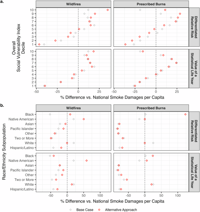
a Damages per capita disparities by overall Social Vulnerability Index decile. Base case estimates are the points from Fig. 2a. Tracts are divided into deciles from least (1) to most (10) vulnerable using Social Vulnerability Index percentile ranks^38,39. b Damages per capita disparities by race/ethnicity. Base case estimates are the diamonds versus the dashed lines in Fig. 6b. a, b Data characterize 2017. Observations are percentage differences versus the national average: $308 per person for wildfire smoke and $313 per person for prescribed burn smoke for the base case. See Supplementary Tables 34–36 for national damages per capita for the alternative approaches. Base case estimates differentiate baseline risk (mortality rates) by race/ethnicity but not relative risk. Base case estimates use a uniform VSL approach ($9.97 million). Alternative approaches differentiate relative risk by race/ethnicity using data from the Medicare Cohort Study³³ and use a VSLY approach ($428 thousand per year)^80,81. See Supplementary Methods 5 for details on the sensitivity analysis of distributional impacts. Plotting uses the ggplot2 R package¹¹⁸.

Full size image

While Fig. 7 indirectly assesses damages by age through its relationship with vulnerability and race/ethnicity (see Supplementary Tables 14 and 15), Fig. 8 explicitly displays the percentage of damages incurred by each age group for each modeling approach. Population percentages are included for reference⁵⁶. While differentiating relative risk had a greater influence when analyzing damages by social vulnerability and race/ethnicity, using the VSLY is intuitively more influential when evaluating damages by age. Interestingly, the interactions between the various inputs to the damage estimates using the VSLY approach still result in senior citizens incurring the lion’s share of damages (55%). This is partially due to the exponential relationship between baseline risk and age (see Supplementary Table 19) and partially related to the fact that we discount the value of future remaining life years—every person’s next year (i.e., 2018) is considered more valuable than a year far into the future (e.g., 2027 or 2037). See Supplementary Tables 34–37 for smoke damages by SVI decile, race/ethnicity, and age group using these different methodologies.

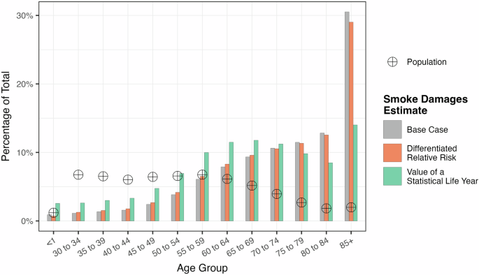
Data characterize 2017. Smoke damage percentages consider both wildfire and prescribed burn emissions. Population percentages consider totals across the contiguous U.S.⁵⁶. Ages 1–29 (38% of the population) experience no damage^18,58. Base case estimates differentiate baseline risk (mortality rates) by race/ethnicity but not relative risk. Base case estimates use a uniform VSL approach ($9.97 million). Alternative approaches differentiate relative risk by race/ethnicity using data from the Medicare Cohort Study³³ and use a VSLY approach ($428 thousand per year)^80,81. See Supplementary Methods 5 for details on the sensitivity analysis of distributional impacts. Plotting uses the ggplot2 R package¹¹⁸.

Full size image

Social vulnerability index

The SVI is provided by the CDC using year-specific data^38,39. The SVIs comprise percentile ranks developed by comparing tracts to one another across 15 social vulnerability variables under four themes, as shown in Table 2. See Supplementary Table 38 for an example of the mathematical computation of percentile ranks. Each variable contributes equal weight to both its theme’s SVI and the overall SVI. We consider rankings nationally, but future work may consider recomputing percentile ranks within more granular boundaries (e.g., regions or states). See Supplementary Methods 3 for more details on the SVI and its use in this study. For SVI percentile ranks at the tract level, see Supplementary Figs. 29 and 30. For trends by regions and states, see Supplementary Table 13 and Supplementary Figs. 4, 9, and 31.

To clarify the role that vulnerability plays in our analysis, we link smoke exposure to vulnerable populations via the tract-level SVI and tract-level PM_2.5 concentration modeling with AP4T. Importantly, our approach does not capture variability within tracts. While baseline mortality risk (the driver of tract-level susceptibility variation for our default modeling) does not directly account for vulnerability as defined by the SVI, it is influenced by factors (e.g., race, age, and geography) that are associated with vulnerability. This alignment ensures that tracts identified as vulnerable via the SVI reflect the corresponding influences on baseline mortality risk and damages per unit of smoke exposure.

Social vulnerability is one of the three domains, along with environmental burden and health vulnerability, of the CDC’s Environmental Justice Index (EJI)¹¹¹. We do not use the EJI for this study because it is only available for 2022. However, even if the EJI were available for 2017, the SVI would still be our preferred index for this study because it incorporates measures of vulnerability that are (at least directly) independent of environmental hazards. This enables us to avoid scenarios where, for instance, vulnerability correlates with smoke impacts because air pollution itself is a vulnerability variable influencing the index. Still, we encourage future work studying emissions-related environmental justice to consider using the EJI in tandem with AP4T.