Stability and control analysis of COVID-19 spread in India using SEIR model

Introduction
One of the most significant global health emergencies of the (21^{st}) century has been the COVID-19 pandemic, caused by the novel coronavirus SARS-CoV-21,2. Emerging in Wuhan, China, towards the end of 2019, this highly contagious virus spread across the globe at an unprecedented rate, prompting some of the most historic public health measures and drastically altering daily life. Commonly referred to as COVID-19, the disease has a broad spectrum of severity, impacting the world in a way that few other crises have3. Recently, Kotola et al.4 investigate the mathematical model for the dynamics of HIV/AIDS and COVID-19 co-infection transmission includes the protection and treatment of both infected and infectious groups. They computer simulations show that the model solutions approach the endemic equilibrium point. Further, Usamn et al.5 uses the Caputo fractional operator with singular kernel to provide a co-dynamical model for COVID-19 and cholera. They numerical evaluations are conducted after determining the model’s optimal order.
SARS-CoV-2 primarily spreads through aerosol transmission, where droplets containing the virus are released into the environment by an infected person during actions such as speaking, coughing, or sneezing. The virus can also spread via fomites, where a contaminated object is touched and then transferred to the face. This easy transmission, coupled with rapid complications, made the virus particularly dangerous. COVID-19 presents a wide variety of symptoms, from mild ones like fever and cough to more severe conditions such as pneumonia and acute respiratory distress syndrome (ARDS). Individuals with pre-existing medical conditions or those who are older are particularly vulnerable to severe outcomes, including hospitalization and death. By July 2024, over 771 million COVID-19 cases had been reported globally, with approximately 6.9 million deaths1,2. Importantly Gudaz et al.6 evaluate a mathematical model that how antiviral treatment affects renal dysfunction. They demonstrated that, depending on the effectiveness of the medicine and its methods of action, therapy might result in either a low or high prevalence. Antiretroviral therapy (ART) for HIV treatment was taken into consideration, Omame et al.7 creating a mechanistic mathematical model. They found that HIV can help mpox spread in MSM communities. Also, HIV can help mpox spread in MSM communities, but ART may not be enough to stop it8.
In India, the pandemic has had profound impacts, directly and indirectly affecting people’s lives. As of July 2024, India has recorded over 77 million confirmed cases and 530,000 deaths. There have been more than 45 million recoveries across the nation1,2. The states most affected include Maharashtra, Kerala, Karnataka, Andhra Pradesh, and Tamil Nadu. For instance, Maharashtra has reported 7.97 million cases, 7.8 million recoveries, and 147,922 deaths, while Kerala has seen 6.6 million cases, 6.5 million recoveries, and 69,993 deaths1,2. In addition, Andhra Pradesh has recorded 2.4 million cases, 2.3 million recoveries, and 15,000 deaths, while Tamil Nadu has reported 3.5 million cases, 3.4 million recoveries, and 99,300 deaths1,2. In order to investigate the effects of prevention and treatment strategies on community transmission, Teklu9 analyzis a mathematical model for the co-infection of the hepatitis B virus and COVID-19. It shows global asymptotically stable points by analyzing local disease-free equilibrium points, boundedness, and model nonnegativity. In addition. Teklu10 investigate the optimal effects of four time-dependent control techniques on the transmission of COVID-19 and HBV.
Governments and health organizations worldwide have implemented various measures to prevent the spread of the virus, including lockdowns, physical distancing, and the use of face masks. The scientific community accelerated vaccine development, and by late December 2020, multiple vaccines received emergency use authorization. These vaccination campaigns have become a cornerstone in efforts to prevent and eventually eliminate the outbreak11. Accordingly, Teklu12 examined the impacts of vaccination, protection measures, hospital and home quarantine tactics, and their qualitative characteristics.
The pandemic has also disrupted economies, education systems, and interpersonal communication. The economic consequences include job losses, shifts in consumer behavior, and changes across industries. Educational institutions faced significant challenges with the sudden shift to online learning, compounded by issues such as unequal access to technology. Social distancing and COVID-19 safety measures significantly altered communication patterns, with many people opting for virtual meetings instead of in-person interactions13.
As the world continues to cope with COVID-19, ongoing research and innovative strategies remain essential. The pandemic has underscored the need for global collaboration and preparedness in addressing emerging diseases. It has also demonstrated the critical importance of flexibility in public health policies to better manage future health risks14. In the context of epidemic modeling, optimal control theory offers a framework to develop intervention strategies that aim to reduce the impact of the disease. By applying tools such as Pontryagin’s Maximum Principle (PMP), optimal control allows us to determine the best strategies to minimize disease spread using interventions such as vaccination (M) and public awareness (p)15.
This study compares three states-Andhra Pradesh, Maharashtra, and Tamil Nadu-between May 1 and May 31, 2020, and uses a mathematical model to analyze the COVID-19 dynamics. The compartmental model is employed to predict the course of the pandemic and create a successful control plan. The study explores the number of infected individuals and control expenses by applying Pontryagin’s maximum principle. According to the study, control measures like immunization can lower infection rates and speed up healing. The study, Also makes recommendations for how lawmakers, government organizations, and health organizations can effectively allocate funds and control the outbreak.
Model formations
The SEIR model, initially developed by Kermack and McKendrick16, is a foundational framework for modeling the spread of infectious diseases. This model divides the population into four distinct compartments: susceptible (S), exposed (E), infectious (I), and recovered (R). In the traditional model, individuals move between compartments based on specific disease parameters. However, for the COVID-19 pandemic in India, several modifications were introduced to capture the impact of public health measures.
The model represents the dynamics of a population in the context of an infectious disease using a compartmental SEIR framework. Each equation describes the rate of change for a particular compartment over time, incorporating parameters for disease transmission, recovery, vaccination, policy interventions, and natural death.
We introduced a time-dependent vaccination parameter, denoted (M(t)), which represents the proportion of the population receiving the vaccine at any given time. Additionally, the model incorporates a public awareness parameter, (p), which simulates the impact of measures such as social distancing and lockdowns on the transmission rate of the virus.
These modifications allow the model to account for dynamic interventions, providing a more realistic simulation of the pandemic’s spread in India. The inclusion of these parameters offers new insights into the effects of vaccination and public awareness campaigns, and demonstrates their importance in managing disease transmission effectively. Simulation results indicate that vaccination efforts significantly reduce the susceptible population, leading to a lower infection rate and a more manageable recovery phase17,18.
The COVID-19 data for Andhra Pradesh, Maharashtra, and Tamil Nadu from May 2020 (Tables 4 and 5), and Table 61,2 provide the foundation for this study’s comparative analysis. These datasets highlight the differences in infection dynamics and serve as input for the SEIR model used in this research.
The parameter values, calculated from the COVID-19 data Tables 4, 5 and 61,2 and summarized in Table 7, were incorporated into the SEIR model to evaluate disease dynamics and intervention strategies.
-
1.
Susceptible population ((S))
-
(A): Recruitment rate, representing the addition of new individuals into the susceptible population (e.g., births or immigration).
-
(-beta S E): Infection rate, reducing susceptibles due to contact with exposed individuals. (beta) is the transmission probability per contact.
-
(-gamma S): Natural death rate, reducing the susceptible population.
-
(-P S M): Vaccination effect, where (P) represents the policy implementation rate, and (M) is the control parameter for vaccination.
Summary: Tracks how susceptibles enter the population (recruitment), get exposed (infection), die naturally, or move to the recovered class via vaccination.
-
2.
Exposed population ((E))
-
(+beta S E): Exposure due to interaction between susceptible and exposed individuals.
-
(-sigma E): Transition of exposed individuals to the recovered class without becoming infectious.
-
(-alpha E): Transition of exposed individuals to the infectious class.
-
(-gamma E): Natural death rate for exposed individuals.
Summary: Describes how the exposed population grows through transmission and decreases through recovery, progression to infectiousness, or death.
-
3.
Infectious population ((I))
-
(+alpha E): Transition of exposed individuals to the infectious class.
-
(-phi I): Recovery rate of infectious individuals, moving them to the recovered class.
-
(-gamma I): Natural death rate among infectious individuals.
Summary: Captures the dynamics of individuals becoming infectious, recovering, or dying due to natural causes while in the infectious state.
-
4.
Recovered population ((R))
-
(+phi I): Recovery of infectious individuals.
-
(+P S M): Contribution of vaccinated individuals transitioning directly to the recovered class.
-
(+sigma E): Recovery of exposed individuals without becoming infectious.
-
(-gamma R): Natural death rate among the recovered population.
Summary: Tracks the growth of the recovered population through recovery (from both infectious and exposed states) and vaccination, while accounting for natural deaths.
Key features of the model
-
Incorporates Vaccination: Terms (P S M) explicitly include the effects of vaccination campaigns. (P) reflects the rate of policy implementation, and (M) measures vaccination control effectiveness.
-
Behavioral Transmission: The infection term (beta S E) accounts for transmission due to contact between susceptibles and exposed individuals, differing from standard SEIR models.
-
Death Rates ((gamma)): Natural death is included in all compartments, reflecting non-disease-related mortality.
-
Policy Relevance: The inclusion of vaccination and policy rates makes the model practical for evaluating public health interventions.
This model extends the classical epidemiological framework by integrating factors such as vaccine administration and heightened public health awareness, as depicted in Fig. 1 and Table 1 describes the description of model parameters. It enables the analysis of the effects of various public health policies and facilitates the identification of the most probable outcomes arising from specific decisions related to COVID-19. The model serves as a tool for understanding the disease’s transmission dynamics and provides guidance for planning measures to mitigate the virus’s impact on the population19.
In this model, (M) represents the proportion of vaccinated individuals transitioning from the (R(t)) category, serving as a measure of vaccine administration. When formulating the optimal control problem, (M) is considered a time-dependent parameter that should be selected to minimize the number of infected individuals. The value of (M(t)) must be bounded between 0 and 1, where 0 indicates no vaccination within the population, and 1 represents maximum vaccination.
Figures 11, 12 and 13: illustrate the impact of varying levels of vaccination implementation (M(t)) on different population compartments during the COVID-19 pandemic over time.
Based on this analysis, a COVID-19 control strategy, as outlined in Fig. 1, is proposed to minimize the number of infected individuals and ensure effective pandemic management.

Schematic Representation of the SEIR Model for the COVID-19 Outbreak in India.
The initial states of the system (1) are (Sleft( 0right) ge 0, Eleft( 0right) ge 0, Ileft( 0right) ge 0, Rleft( 0right) ge 0).
Bounded solutions
Now, we define the total population (Y = S + E + I + R), representing the sum of all compartments. Differentiating (Y) with respect to time gives3,20:
Substituting the expressions for (frac{dS}{dt}), (frac{dE}{dt}), (frac{dI}{dt}), and (frac{dR}{dt}), we get:
After simplifying, the terms involving (beta S E), (alpha E), (phi I), and (P S M) cancel out, leaving:
This simplifies to:
Solving the Differential Equation
This is a first-order linear differential equation. We solve it using separation of variables:
Integrating both sides:
The left-hand side becomes:
Solving for (Y):
Solving for (Y):
Determining the Constant (C_2)
Using the initial condition (Y(0) = Y_0), we have:
Solving for (C_2):
Thus, the solution for (Y(t)) is:
Asymptotic Behavior
As (t rightarrow infty), (e^{-gamma t} rightarrow 0), so the solution approaches:
Boundedness and Stability
From the equation:
we conclude that (Y(t)) is bounded and will stabilize at (frac{A}{gamma }). This shows that the total population will not grow indefinitely and will reach a steady-state value. The boundedness of the solutions was confirmed using initial conditions derived from Tables 4, 5 and 61,2 which provide state-specific data on infection dynamics.Thus, the solutions of the nonlinear equation system remain uniformly bounded and the system is stable in the long run3,20.
Transmission potential of COVID-19
The Transmission potential metric ((R_0)) is crucial in comprehending the spread of diseases, as it signifies the average number of subsequent cases generated by a single infected person during their entire infectious period3,11,20,21.
The system can be represented as:
where
A system of nonlinear differential equations (1) governs the dynamics of the SEIR model, comprising:
A state of equilibrium without disease can be achieved. The Jacobian matrices of the functions (phi) and (psi) evaluated at this disease-free equilibrium point, are given by:
Then
The basic reproduction number, (R_0), which is also known as the spectral radius of the matrix, is a critical element in the model presented, described by the expression (F V^{-1}). This parameter represents the average number of secondary cases generated by a single individual during their infectious period. The contour plot of (R_0) in relation to the disease transmission rate ((beta)) and the COVID-19 fatality rate ((gamma)) is shown in Figs. 2 and 3 and 4, while the surface plot of (R_0) concerning (beta) and (gamma) is displayed in Figs. 5, 6 and 7, Using parameter values from Table 7, the reproduction number (R_0) was calculated for Andhra Pradesh, Maharashtra, and Tamil Nadu, enabling comparative analysis across states.
-
Figure 2: This figure represents a 2D graphical plot for the state of Andhra Pradesh. The plot shows the relationship between the reproduction number (R_0), the disease transmission rate (beta), and the COVID-19 fatality rate (gamma). This helps visualize how variations in these parameters affect the basic reproduction number for Andhra Pradesh.
-
Figure 3: Similar to Fig. 2, this plot is for the state of Maharashtra. The plot represents the same relationship between (R_0), (beta), and (gamma) but for Maharashtra. The key difference here is that the parameters specific to Maharashtra are used, reflecting the state’s particular conditions.
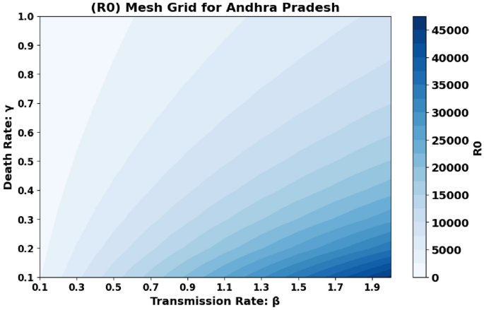
Andhra Pradesh State Graphical representation of (R_0) in relation to disease transmission rate ((beta )) and COVID-19 fatality rate ((gamma )).
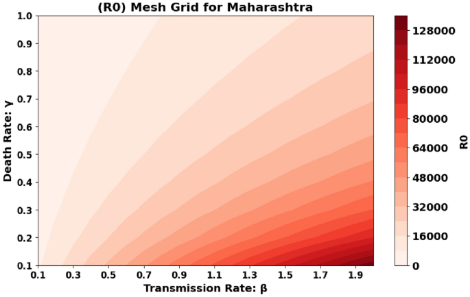
Maharashtra State Graphical representation of (R_0) in relation to disease transmission rate ((beta )) and COVID-19 fatality rate ((gamma )).
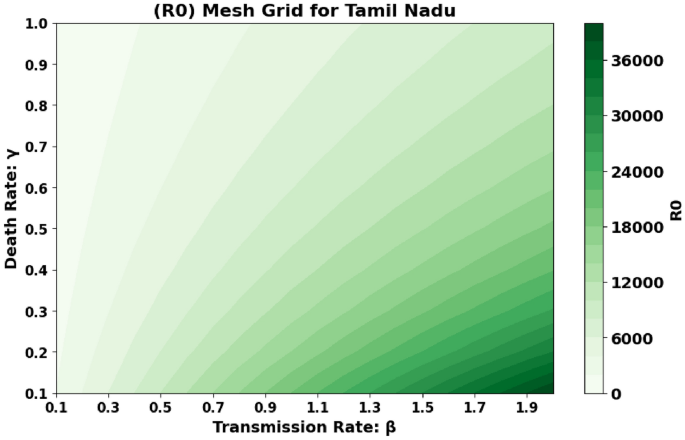
Tamil Nadu State Graphical representation of (R_0) in relation to disease transmission rate ((beta )) and COVID-19 fatality rate ((gamma )).
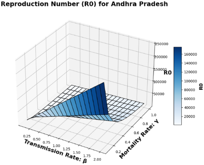
Andhra Pradesh State Surface plot of (R_0) in relation to the Disease Transmission Rate ((beta )) and the COVID-19 Mortality Rate ((gamma )).
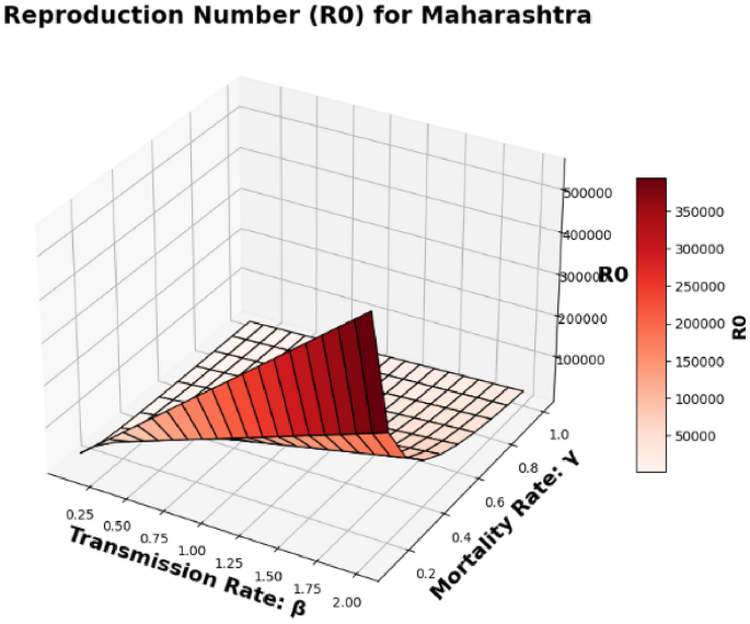
Maharashtra State Surface plot of (R_0) in relation to the Disease Transmission Rate ((beta )) and the COVID-19 Mortality Rate ((gamma )).
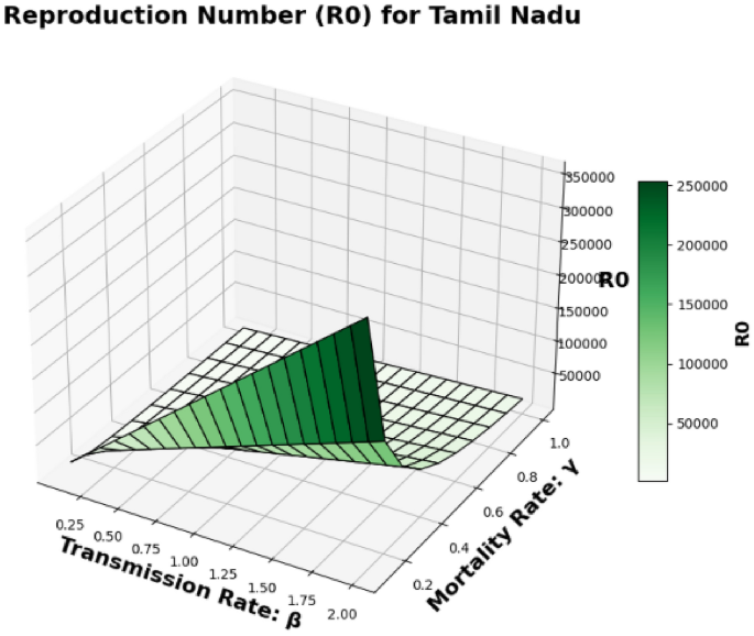
Tamil Nadu State Surface plot of (R_0) in relation to the Disease Transmission Rate ((beta )) and the COVID-19 Mortality Rate ((gamma )).
-
Figure 4: This figure shows the same graphical representation of (R_0) but for Tamil Nadu. The plot depicts how the transmission rate (beta) and fatality rate (gamma) influence the reproduction number (R_0) for this state. It helps compare the dynamics of disease spread in Tamil Nadu to those in Andhra Pradesh and Maharashtra.
-
Figure 5: This figure presents a 3D surface plot for Andhra Pradesh. Unlike the previous 2D plots, this surface plot shows how the reproduction number (R_0) is affected by both the disease transmission rate (beta) and the COVID-19 mortality rate (gamma) in a 3D context. This provides a more comprehensive view of the relationship between the parameters in Andhra Pradesh.
-
Figure 6: Similar to Fig. 5, this is a 3D surface plot, but for the state of Maharashtra. It shows how (R_0) varies with both (beta) and (gamma) in Maharashtra. This plot highlights the state’s specific reproduction number dynamics based on the disease transmission rate and the mortality rate.
-
Figure 7: This is another surface plot, but this one is for Tamil Nadu. Like Figs. 5 and 6, it shows the relationship between (R_0), (beta), and (gamma) in a 3D context, but for Tamil Nadu. This surface plot provides a visual representation of how these parameters affect the basic reproduction number in Tamil Nadu.
State-wise comparison
Andhra Pradesh (AP)
-
May 2020 (R_0) Value: 0.1930
-
Trend: Increasing
In Andhra Pradesh, the (R_0) value of 0.1930 in May 2020 indicates that each infected person was transmitting the virus to approximately 0.19 other individuals. The increasing trend suggests a rise in community transmission, highlighting a growing spread of the virus.
Maharashtra (MH)
-
May 2020 (R_0) Value: 0.2170
-
Trend: Increasing
Maharashtra recorded a higher (R_0) value of 0.2170, indicating a faster rate of transmission compared to Andhra Pradesh. The increasing trend reflects a significant rise in cases, consistent with the state’s early heavy burden during the pandemic, especially in metropolitan areas like Mumbai.
Tamil Nadu (TN)
-
May 2020 (R_0) Value: 0.0334
-
Trend: Increasing
Tamil Nadu had the lowest (R_0) value of 0.0334 in May 2020. This suggests that the virus was spreading more slowly compared to Maharashtra and Andhra Pradesh, which could be attributed to more effective containment measures. However, the increasing trend indicates that the spread was accelerating over time.
-
Maharashtra exhibited the highest (R_0) value in May 2020 (0.2170), followed by Andhra Pradesh (0.1930), and Tamil Nadu (0.0334).
-
The increasing (R_0) values across all three states suggest growing community transmission during this period.
-
Maharashtra, with a dense population and high urbanization, faced a more rapid outbreak, while Tamil Nadu’s lower (R_0) suggests relatively better initial control of the virus.
In May 2020, the (R_0) values for Maharashtra, Andhra Pradesh, and Tamil Nadu reflected differing rates of COVID-19 transmission. Maharashtra experienced the highest (R_0), signaling a rapid spread, while Andhra Pradesh showed a moderate increase. Tamil Nadu had a lower (R_0), suggesting a slower spread, though the increasing trend indicated a rising transmission rate. These differences underscore the varied impact of COVID-19 across states in India during the early phase of the pandemic.
Stable states
The system has two stable states: the healthy equilibrium, (E_0(S_0,0,0,R_0)), where no disease is present, and the endemic steady state, (E_1(S^*,E^*,I^*,R^*)), where the infection is continually present, and the disease is endemic3,20.
Where (S_0 = frac{textit{A}}{gamma + P M}), (R_0 = frac{A beta }{(gamma +P M) (sigma + alpha + gamma )}) and the other one is endemic equilibrium point in this endemic equilibrium the infections present always and gives (E_1 (S^*,E^*,I^*,R^* )) and graphical representation of endemic equilibrium is shown in Figs. 26, 27, 28, 29, 30, 31, 32, 33, 34, 35, 36 and 37.
Local asymptotic stability (DFE)
We evaluated the local asymptotic stability of the Healthy State Equilibrium and Persistent Infection Equilibrium. Our analysis revealed that the Healthy State Equilibrium (E_0) is stable for (R_0 < 1), but loses stability when (R_0 > 1)3,11,20,21. The Jacobian matrix associated with the Healthy State Equilibrium of the nonlinear system (1), At the DFE, we have22,23:
The Jacobian matrix for the system is given by:
To determine the local stability of the DFE, we compute the eigenvalues of (J). Subtracting (lambda) from the diagonal elements gives (J – lambda I):
The determinant of (J – lambda I) is computed as:
Characteristic Equation
The Jacobian matrix is block triangular, so the determinant can be split into components:
Top-left 2×2 block:
Bottom-right 2×2 block:
Final Characteristic Equation:
Combining all components, the characteristic equation is:
Routh-Hurwitz Stability Analysis
To analyze the stability of the system, we use the characteristic polynomial:
The coefficients of the polynomial are given by:
Using the Routh-Hurwitz criterion, we construct the Routh table as follows:
-
The first element in the Routh array is defined as:
$$begin{aligned} a_3 = a_1 end{aligned}$$(This represents the relationship between the first and third coefficients of the polynomial.)
-
The second element in the Routh array is defined as:
$$begin{aligned} a_2 = a_0 end{aligned}$$(This corresponds to the second and zeroth coefficients in the polynomial.)
-
The next element, (b_1), is calculated as:
$$begin{aligned} b_1 = frac{a_2 a_1 – a_3 a_0}{a_2} end{aligned}$$(This uses a determinant-like formula to compute the third row value in the Routh array.)
-
The element (c_1) is determined using:
$$begin{aligned} c_1 = frac{b_1 a_0}{b_1} end{aligned}$$(This uses the value of (b_1) and the zeroth coefficient to calculate the fourth row element.)
For the system to be locally asymptotically stable, the following conditions must hold:
Substituting (S_0 = frac{A}{gamma + PM}) Using the equilibrium value of (S_0), substitute into the coefficients where (S_0) appears. The system is stable if all coefficients of the first column in the Routh table are positive. If the Routh-Hurwitz stability conditions are satisfied, the disease-free equilibrium (DFE) is locally asymptotically stable. This implies that, in the absence of perturbations, the system will converge to the DFE, and the disease will die out over time and graphical representation of disease free equilibrium is shown in Figs. 14, 15, 16, 17, 18, 19, 20, 21, 22, 23, 24 and 25, Data-driven parameter values Table 7 were used to determine the local stability of the Disease-Free Equilibrium (DFE) in the three states.
Local asymptotic stability (EE)
At the Endemic Equilibrium (EE), the steady-state values are:
Jacobian matrix at EE
The Jacobian matrix for the system at the EE is:
Subtracting (lambda) from the diagonal elements, we have:
Characteristic equation
The determinant of (J – lambda I) is:
The matrix is block triangular, so the determinant becomes:
Final Characteristic Equation:
Combining all components, the characteristic equation is:
The characteristic polynomial is:
where the coefficients are:
Routh-Hurwitz stability analysis
Using the Routh-Hurwitz criterion, construct the Routh table as follows:
-
The element (a_3) is defined as:
$$begin{aligned} a_3 = a_1 end{aligned}$$(This represents the relationship between the first and third coefficients of the polynomial.)
-
The element (a_2) is defined as:
$$begin{aligned} a_2 = a_0 end{aligned}$$(This corresponds to the second and zeroth coefficients in the polynomial.)
-
The element (b_1) is calculated as:
$$begin{aligned} b_1 = frac{a_2 a_1 – a_3 a_0}{a_2} end{aligned}$$(This formula is used to compute the third value in the Routh array.)
-
The element (c_1) is determined using:
$$begin{aligned} c_1 = frac{b_1 a_0}{b_1} end{aligned}$$(This uses the value of (b_1) and the zeroth coefficient to calculate the fourth value in the Routh array.)
The system is locally asymptotically stable at the EE if:
By substituting the equilibrium values (S^*, E^*, I^*, R^*) into the coefficients, verify the Routh-Hurwitz conditions. If all conditions are satisfied, the Endemic Equilibrium (EE) is locally asymptotically stable, indicating the disease persists in the population at steady levels and graphical representation of endemic equilibrium is shown in Figs. 26, 27, 28, 29, 30, 31, 32, 33, 34, 35, 36 and 37, The analysis of the endemic equilibrium state incorporates parameter values from Table 7, derived from Tables 4, 5 and 61,2 reflecting the persistence of infections in Andhra Pradesh, Maharashtra, and Tamil Nadu.
Sensitivity analysis
This section investigates the impact of parameter value modifications on the reproduction number’s functional value. Identifying the key parameter that acts as a threshold for disease control is essential. The sensitivity indices for20,24
The normalized sensitivity index of a parameter (x) is defined as:
and with respect to the parameters (beta ,gamma ,alpha ,sigma) are calculated as follows:
The fact that all partial derivatives are positive suggests that R(_{0}) is directly influenced by each of the mentioned factors. By examining the proportional responses to proportional changes, we can gain insights into the elasticity of R(_{0}) with respect to these factors20,Sensitivity analysis of (R_0) was conducted using parameters derived from Table 7, which summarize key factors like (beta), (alpha), (phi), and (sigma) based on state-specific data from Tables 4, 5 and 61,2.
(R_0) Values for Each State:
-
Andhra Pradesh: (R_0 = 0.193)
-
Maharashtra: (R_0 = 0.217)
-
Tamil Nadu: (R_0 = 0.033)
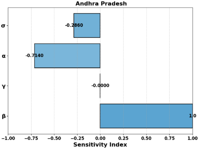
Sensitivity Index of (R_0) for Andhra Pradesh.
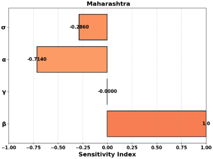
Sensitivity Index of (R_0) for Maharashtra.
Sensitivity Index of (R_0) for Tamil Nadu.
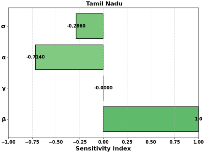
Sensitivity indices ((E_x)) summary
Figures 8, 9, and 10 represent the sensitivity indices of the basic reproduction number, (R_0), for three different states: Andhra Pradesh, Maharashtra, and Tamil Nadu, respectively and Table 2 highlights the sensitivity indices for the parameters influencing (R_0) providing a detailed comparative analysis across the states.
In Fig. 8, the sensitivity indices show how various parameters influence the basic reproduction number (R_0) in Andhra Pradesh. The most significant effect is seen with the parameter (beta), which has a positive sensitivity index of 1, indicating that an increase in (beta) (transmission rate) directly increases (R_0). Conversely, the parameters (sigma), (alpha), and (gamma) have negative sensitivity indices, implying that their increases would decrease the value of (R_0).
Figure 9 presents the sensitivity indices for Maharashtra. The parameter (beta) shows a similar trend to Andhra Pradesh, with a positive sensitivity index of 1, highlighting its direct role in increasing (R_0). (sigma) and (alpha) have negative indices, again indicating that their increases reduce (R_0). The sensitivity of (gamma) is near zero, indicating its minimal effect on the reproduction number in this state.
Figure 10 displays the sensitivity index of (R_0) for Tamil Nadu. The sensitivity indices for Tamil Nadu are similar to those of Andhra Pradesh and Maharashtra, where (beta) has the largest effect on (R_0). (sigma), (alpha), and (gamma) contribute negatively to (R_0), and the effect of (phi) is negligible.
These figures highlight the relative importance of various epidemiological parameters in influencing the basic reproduction number, which is crucial for understanding disease transmission dynamics and guiding intervention strategies in each state.
-
Positive Sensitivity: Parameters (beta) and (A) exhibit a sensitivity of (1.0), showing a direct proportional relationship with (R_0).
-
Negative Sensitivity: Parameters (gamma , M,) and (P) have negative sensitivities, indicating an inverse relationship with (R_0). Notably, (S_M) and (S_P) are very close to (-1.0), making them highly sensitive.
-
Moderate Negative Sensitivity: Parameters (alpha) and (sigma) have moderate negative sensitivities ((-0.714) and (-0.286), respectively).
Optimal intervention strategies of vaccine administration
The optimal control strategy for COVID-19 vaccination in India, specifically in states like Tamil Nadu, Andhra Pradesh, and Maharashtra, focuses on maximizing the public health benefits by minimizing the spread of the virus and reducing the healthcare burden. The Indian government has implemented a phased vaccination strategy, prioritizing healthcare workers, senior citizens, and individuals with comorbidities in the early stages, followed by the general population. The vaccination campaigns in these states are designed using an optimal control framework, which helps balance the number of people vaccinated with the available vaccine supply, public health infrastructure, and societal factors, Optimal control strategies were evaluated using the vaccination parameter ((M)) and other values from Table 7, derived from May 2020 data Tables 4, 5 and 61,2 for each state.
The objective of the strategy is to minimize the infection rates while ensuring that the vaccination rollout occurs efficiently. Optimal control models often incorporate factors such as the rate of vaccine distribution, population density, and behavioral responses, which vary across different regions. For instance, in Tamil Nadu and Andhra Pradesh, the focus has been on addressing rural areas with limited access to healthcare services, while Maharashtra, with its larger urban centers like Mumbai, emphasizes reaching a high-density population. Moreover, the strategy also considers the challenges of vaccine hesitancy and the logistics involved in maintaining cold-chain supply lines. The goal is to achieve herd immunity as quickly as possible while avoiding system overload, and these strategies are continually adjusted as new data and variants of the virus emerge3,22,25,26.
By applying optimal control theory, the government can evaluate the impact of different vaccination rates, the timing of interventions, and the effects of lockdowns or other non-pharmaceutical interventions to decide on the best course of action, thus improving both the economic and health outcomes in these states15,20,27.
In this context, M(t) represents the implementation of vaccine administration as a time-varying control strategy, which was introduced by the Indian government to raise awareness about vaccination in public places. This initiative has proven to be crucial in recent times, as it significantly reduces the transmission of the virus among individuals. To develop such a strategy, we can employ optimal control theory, aiming to minimize the spread of the virus. The primary objective of the optimal control problem is to determine the optimal vaccine administration strategy that minimizes virus transmission. We can formulate the objective function as follows:19,21
Let the state variables of the system be denoted by (S(t)), (E(t)), (I(t)), and (R(t)), which represent the susceptible, exposed, infected, and recovered individuals, respectively. The system dynamics are given by the following set of differential equations:
Here, (A) is a constant representing the population inflow, (beta) is the transmission rate, (gamma) is the natural death rate, (P) is a vaccination rate parameter, (M) is the vaccination coverage, (sigma) is the rate of progression from exposed to infected, (alpha) is the rate of infection-induced death, and (phi) is the recovery rate. The state variables evolve over time as governed by these equations23.
The objective is to minimize a cost function (J), which typically consists of terms that represent the benefits of the control (e.g., reducing the number of infections) and the costs of the control (e.g., the cost of administering the vaccine). For example, the cost function can be written as:
Given the model specified in Equation (c_1) is the coefficient corresponding to the infected population and (c_2) is a controlled parameter with limited bounds. The functional is linear and its values are restricted within predetermined limits.
Furthermore, we can leverage established results to guarantee optimal control and suitable optimal states23,24. The objective is to find the optimal control value M(t) such that it minimizes or maximizes the desired outcome, subject to the constraints of the system.
To find the optimal control, we apply Pontryagin’s Maximum Principle, which provides the necessary conditions for optimality. The principle states that for an optimal control problem, the optimal control (mathbf {lambda }^*(t)) must maximize the Hamiltonian. This gives the condition22,23:
The next step is to define the Hamiltonian (mathscr {G}), which incorporates the system dynamics and the objective function. The Hamiltonian is given by:
where (lambda _1(t), lambda _2(t), lambda _3(t), lambda _4(t)) are the costate variables (also called adjoint variables), and (L(S, E, I, R, mathbf {lambda }(t))) is the running cost, which may include both the state and control costs and the costate equations, which are obtained by differentiating the Hamiltonian with respect to the state variables22:
The solution to these equations, along with the boundary conditions, provides the optimal trajectory of the system state and costates28.
We aim to optimize the control variable M(t) to minimize the Hamiltonian. Notably, the Hamiltonian exhibits linearity with respect to the control parameter, indicating a singular optimal control. Consequently, the switching function can be expressed as22
If the switching function becomes zero on a non-trivial interval of time, then singular control occurs. In this case, the optimal control strategy is to set the control variable at its upper bound or lower bound, depending on whether the switching function is positive or negative, respectively, on the adjacent intervals, (frac{partial mathscr {G}}{partial M}<0 or >0) to verify the singular case, we may assume that (frac{partial mathscr {G}}{partial M}=0)
For a certain non-trivial time interval, we compute the time derivative of the partial derivative of (mathscr {G}) with respect to M, setting it equal to zero: (frac{d}{dt}left( frac{partial mathscr {G}}{partial M}right) =0). After simplifying the expression for the time derivative of (frac{partial mathscr {G}}{partial M}), we arrive at
Using the system of equations 1 we obtain
The absence of the control parameter M in the given equations necessitates the calculation of the second-order time derivative. This additional step is required to gain insights into the system’s behavior, as the control parameter’s influence is not directly apparent.
The aforementioned equation can be expressed in the following form
And the we solve the singular control as (M_{Singular; } left( tright) =; -frac{varphi _{2} left( tright) }{varphi _{1} left( tright) })
Provided (; ; varphi _{1} left( tright) ; ne 0; and; ale ; -frac{varphi _{2} left( tright) }{varphi _{1} left( tright) } le b), Where
And
Additionally, the equation needs to fulfill the Generalized Legendre-Clebsch criterion, expressed as
(frac{d^{2} }{dt^{2} } left( frac{partial mathscr {G}}{partial M} right) =varphi _{1} left( tright)) To be negative, the conclusion part of control profile is defined by If (frac{partial mathscr {G}}{partial M} <0,; ; then; M^{*} left( tright) =b;) If (frac{partial mathscr {G}}{partial M} >0,; ; then; M^{*} left( tright) =a) If (frac{partial mathscr {G}}{partial M} =0,; ; then; M_{Singular; } left( tright) =; -frac{varphi _{2} left( tright) }{varphi _{1} left( tright) })
Hence the Control optimal provided (varphi _{1} left( tright) <0; ; ; and; ; ; ale -frac{varphi _{2} left( tright) }{varphi _{1} left( tright) } le b).
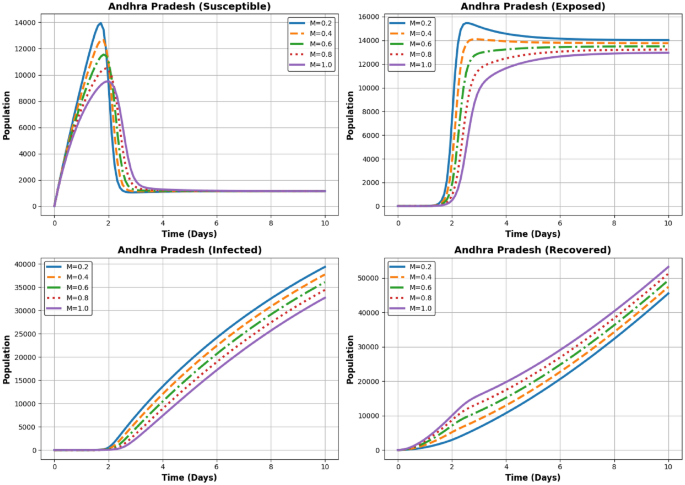
Dynamics of the Susceptible, Exposed, Infected, and Recovered populations for different (M) values ((M = 0.2, 0.4, 0.6, 0.8, 1.0)) in Andhra Pradesh.
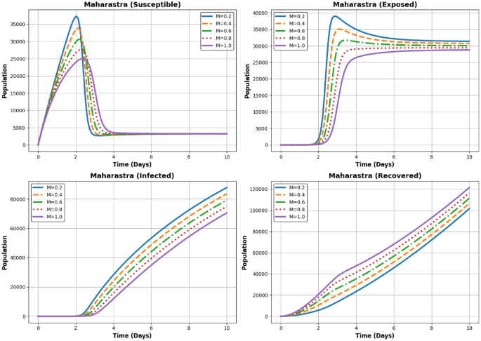
Dynamics of the Susceptible, Exposed, Infected, and Recovered populations for different (M) values ((M = 0.2, 0.4, 0.6, 0.8, 1.0)) in Maharastra.
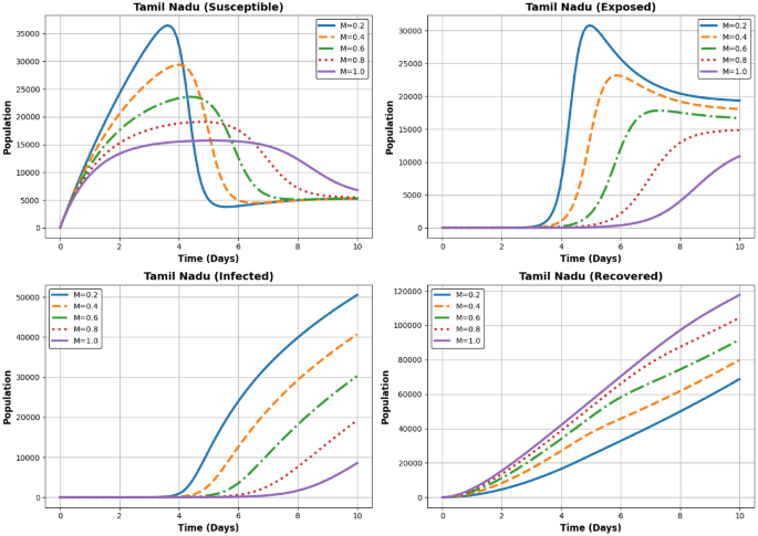
Dynamics of the Susceptible, Exposed, Infected, and Recovered populations for different (M) values ((M = 0.2, 0.4, 0.6, 0.8, 1.0)) in Andhra Pradesh Tamil Nadu.
Figures 11, 12 and 13 illustrates the impact of different levels of vaccination implementation (M(t)) at three states AP, Maharastra and TN, where (M) represents the intensity of the vaccination effort over time during the COVID-19 pandemic. Finally, after solving for the optimal control, we analyze the results. This involves checking if the control strategy achieves the desired objectives (e.g., minimizing infections while controlling costs) and whether it is feasible in practice. Sensitivity analysis can also be performed to understand how changes in the parameters (e.g., vaccination rates, budget) affect the optimal control strategy.
In Fig. 11 the Susceptible population declines rapidly with higher (M). This demonstrates the impact of increased recovery efforts and better containment measures. The Exposed population follows a pattern similar to Andhra Pradesh, with a sharp peak followed by a gradual decline. Higher (M) values result in a faster reduction in exposure, The Infected population peaks before reducing over time. For higher (M), the peak is significantly lower, and the decline is faster, suggesting better management of the disease spread, The Recovered population shows a steady increase, with higher (M) leading to quicker recovery rates and a larger final recovered population, The exposed and infected populations decline faster with higher (M), indicating effective recovery dynamics in Andhra Pradesh.
In Fig. 12 the Susceptible population declines rapidly with higher (M). This demonstrates the impact of increased recovery efforts and better containment measures. The Exposed population follows a pattern similar to Andhra Pradesh, with a sharp peak followed by a gradual decline. Higher (M) values result in a faster reduction in exposure. The Infected population peaks before reducing over time. For higher (M), the peak is significantly lower, and the decline is faster, suggesting better management of the disease spread. The Recovered population shows a steady increase, with higher (M) leading to quicker recovery rates and a larger final recovered population. The exposed and infected populations decline faster with higher (M), indicating effective recovery dynamics in Maharashtra.
In Fig. 13 the Susceptible population decreases rapidly for higher (M) values, as recovery efforts divert individuals to the recovered category faster. The Exposed population peaks early and declines quickly for higher (M), following similar dynamics to Andhra Pradesh and Maharashtra. The Infected population’s peak height decreases with increasing (M). Faster declines are observed for higher (M), emphasizing the importance of recovery dynamics. The Recovered population increases steadily over time. Higher (M) leads to faster recovery and a larger final recovered population. The population dynamics in Tamil Nadu follow similar trends to Andhra Pradesh and Maharashtra, with slight variations due to regional differences.
Numerical analysis
The SEIR (Susceptible-Exposed-Infectious-Recovered) model provides a framework for analyzing the spread of COVID-19 across different regions by categorizing the population into four compartments. This analysis incorporates data from Tamil Nadu, Maharashtra, and Andhra Pradesh, focusing on endemic equilibrium states and sensitivity indices of key parameters.
At equilibrium, the state variables-susceptible ((S^*)), exposed ((E^*)), infectious ((I^*)), and recovered ((R^*))-reach stable values under constant parameters. Table 1 lists the results for each region:
The basic reproduction number ((R_0)) varies by region, with values of 0.0334 for Tamil Nadu, 0.2170 for Maharashtra, and 0.1930 for Andhra Pradesh, indicating differing levels of disease transmission potential across states. Sensitivity indices highlight the influence of parameters on (R_0), providing insights into prioritizing control strategies (Table 3). Table 2 shows these indices for (beta), (gamma), (alpha), and (sigma).
The SEIR model effectively captures regional variations in COVID-19 dynamics, aiding in understanding disease progression and optimizing intervention strategies. Sensitivity analysis underscores the importance of reducing the transmission rate ((beta)) through policies such as social distancing, mask mandates, and vaccination programs. Further exploration of control parameters ((P, M)) can refine strategies for sustainable epidemic management, The findings, informed by COVID-19 data from Tables 4, 5 and 61,2 and parameter estimates in Table 7, underline the need for state-specific interventions to effectively reduce infection rates and mitigate the pandemic’s impact.
In Table 3, the Endemic Equilibrium States for Tamil Nadu, Maharashtra, and Andhra Pradesh are shown, highlighting key differences in the equilibrium values for susceptible, exposed, infected, and recovered populations. These differences reflect the impact of regional factors such as population density, healthcare response, and intervention measures.
In this study, we analyze the dynamics of the susceptible ((S)), exposed ((E)), infected ((I)), and recovered ((R)) populations across three states in India, namely Andhra Pradesh, Maharashtra, and Tamil Nadu. The results from the numerical simulations are presented in Figs. 14, 15, 16, 17, 18, 19, 20, 21, 22, 23, 24 and 25, which illustrate the progression of these populations over time.
-
Susceptible Population Dynamics (DFE): As shown in Figs. 14, 15 and 16, the susceptible population in Andhra Pradesh, Maharashtra, and Tamil Nadu follows distinct trends due to varying transmission rates and public health interventions.
-
Exposed Population Dynamics (DFE): Figures 17, 18 and 19 present the evolution of the exposed population. While Andhra Pradesh experiences a gradual increase, Maharashtra sees a sharper rise, as depicted in Fig. 18.
-
Infected Population Dynamics (DFE): The infected population follows a more dramatic trajectory in Maharashtra, as shown in Figs. 21 and 22.
-
Recovered Population Dynamics (DFE): The recovered population trends are shown in Figs. 23, 24 and 25, with Tamil Nadu exhibiting a steady rise in recoveries compared to the other two states.
In this study, we examine the dynamics of the endemic equilibrium (EE) across Andhra Pradesh, Maharashtra, and Tamil Nadu. The results from the numerical simulations are shown in Figs. 26, 27, 28, 29, 30, 31, 32, 33, 34, 35, 36 and 37, which depict the dynamics of the susceptible, exposed, infected, and recovered populations at the endemic equilibrium.
-
Susceptible Population Dynamics (EE): As shown in Figs. 26, 27 and 28, the susceptible population across all three states reaches an equilibrium value.
-
Exposed Population Dynamics (EE): The exposed population, as shown in Figs. 29, 30 and 31, behaves differently in each state at EE.
-
Infected Population Dynamics (EE): Figures 32, 33 and 34 illustrate the stabilization of the infected population in each state at EE.
-
Recovered Population Dynamics (EE): The recovered population reaches a steady state, as illustrated in Figs. 35, 36 and 37.
Parameter definitions and estimations
The following parameters are used in the epidemiological model to estimate the dynamics of disease transmission. The values provided are state-specific, based on recent data and public health policies. These values are crucial for adjusting the model to accurately reflect the disease’s behavior in different states of India.
-
A (Rate of new recruitment into the susceptible population): The recruitment rate into the susceptible population, A, is determined by birth rates, migration, and other factors. This can be approximated as:
$$begin{aligned} A = text {Population Growth Rate} times N_{text {Total}} end{aligned}$$where (N_{text {Total}}) is the total population size.
-
M (Optimal control parameter for vaccine administration): The vaccination rate, denoted by M, is influenced by the proportion of the population vaccinated and the effectiveness of vaccination programs:
$$begin{aligned} M = frac{V_{text {administered}}}{N_{text {total}}} end{aligned}$$where (V_{text {administered}}) is the total number of vaccines administered during a specific period, and (N_{text {total}}) is the total population.
Estimated values for the states are:
-
Tamil Nadu: (M approx 0.8 , text {to} , 1.0)
-
Andhra Pradesh: (M approx 0.7 , text {to} , 0.9)
-
Maharashtra: (M approx 0.9 , text {to} , 1.1)
-
-
P (Rate of policy enforcement): The rate of policy enforcement, P, is the effectiveness of control measures such as lockdowns and social distancing. It can be modeled as:
$$begin{aligned} P = frac{C_{text {total}}}{N_{text {total}}} end{aligned}$$where (C_{text {total}}) represents the cumulative effect of control measures (e.g., percentage of people adhering to lockdowns, wearing masks), and (N_{text {total}}) is the total population. Estimated values for the states are:
-
Tamil Nadu: (P approx 0.4 , text {to} , 0.6)
-
Andhra Pradesh: (P approx 0.3 , text {to} , 0.5)
-
Maharashtra: (P approx 0.7 , text {to} , 0.9)
-
-
(beta) (Probability of disease transmission per contact): The transmission rate (beta) represents the probability that a susceptible individual will become infected after contact with an infected individual. It is typically modeled as:
$$begin{aligned} beta = frac{D_{text {new}}}{S_{text {total}} times I_{text {total}}} end{aligned}$$where (D_{text {new}}) is the number of new cases, (S_{text {total}}) is the number of susceptible individuals, and (I_{text {total}}) is the number of infectious individuals.
-
(sigma) (Rate of progression or recovery from the exposed class): The rate (sigma) indicates how quickly individuals in the exposed class (latent) progress to being infectious or recover. This is typically estimated based on disease progression studies:
$$begin{aligned} sigma = frac{1}{text {Incubation Period}} end{aligned}$$ -
(alpha) (Rate at which individuals progress from the exposed to the infectious class): The rate (alpha) quantifies how fast individuals transition from the exposed class to the infectious class, which can be modeled as:
$$begin{aligned} alpha = frac{1}{text {Incubation Period}} end{aligned}$$This is similar to (sigma) but emphasizes progression to the infectious stage.
-
(phi) (Recovery rate from the infectious to the recovered class): The recovery rate (phi) indicates how quickly individuals recover after being infected:
$$begin{aligned} phi = frac{1}{text {Recovery Period}} end{aligned}$$ -
(gamma) (Natural mortality rate): The natural mortality rate (gamma) represents the baseline death rate in the population unrelated to the disease. This is typically based on demographic data and is assumed to be constant across populations:
$$begin{aligned} gamma = frac{text {Total Deaths}}{text {Population}} end{aligned}$$
Summary table
The following Figs. 14, 15, 16, 17, 18, 19, 20, 21, 22, 23, 24 and 25 focusing on the dynamics of the (S), (E), (I), and (R) compartments across Andhra Pradesh, Maharashtra, and Tamil Nadu.
-
Figures 14, 15 and 16: Susceptible Population
-
Figure 14: Susceptible Population in Andhra Pradesh. The susceptible population ((S)) starts high and decreases rapidly as individuals become exposed or infected, stabilizing by the end of the period.
-
Figure 15: Susceptible Population in Maharashtra. The susceptible population ((S)) shows a similar rapid decline, with a greater initial decrease compared to Andhra Pradesh, reflecting higher transmission rates.
-
Figure 16: Susceptible Population in Tamil Nadu. The susceptible population ((S)) decreases more slowly compared to the other states, reflecting slower transmission dynamics.
-
-
Figures 17, 18 and 19: Exposed Population
-
Figure 17: Exposed Population in Andhra Pradesh. The exposed population ((E)) initially increases, then decreases as individuals transition to infected or recovered states.
-
Figure 18: Exposed Population in Maharashtra. The exposed population ((E)) increases sharply, reflecting faster transmission, before eventually declining.
-
Figure 19: Exposed Population in Tamil Nadu. The exposed population ((E)) grows moderately, then plateaus, indicating effective containment and lower transmission rates.
Fig. 14 
DFE – Andhra Pradesh State – Susceptible population (S).
Fig. 15 
DFE – Maharashtra State – Susceptible population (S).
Fig. 16 
DFE – Tamil Nadu State – Susceptible population (S).
Fig. 17 
DFE – Andhra Pradesh State – Exposed population (E).
Fig. 18 
DFE – Maharashtra State – Exposed population (E).
Fig. 19 
DFE – Tamil Nadu State – Exposed population (E).
Fig. 20 
DFE – Andhra Pradesh State – Infected population (I).
Fig. 21 
DFE – Maharashtra State – Infected population (I).
Fig. 22 
DFE – Tamil Nadu State – Infected population (I).
Fig. 23 
DFE – Andhra Pradesh State – Recovered population (R).
Fig. 24 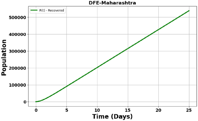
DFE – Maharashtra State – Recovered population (R).
Fig. 25 
DFE – Tamil Nadu State – Recovered population (R).
Fig. 26 
EE – Andhra Pradesh State – Susceptible population (S).
Fig. 27 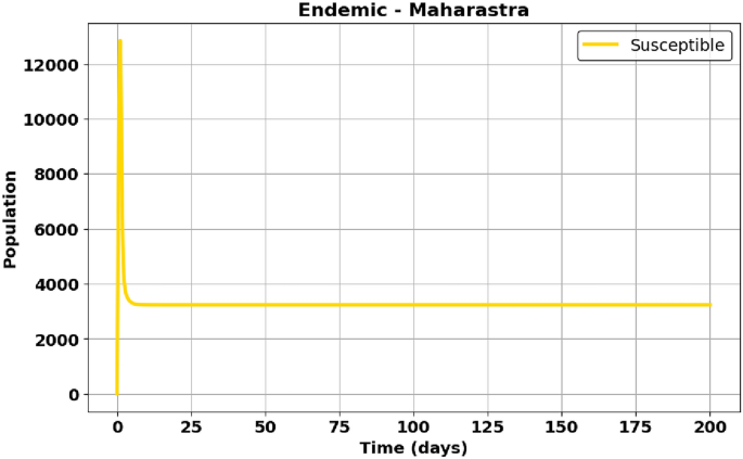
EE – Maharashtra State – Susceptible population (S).
Fig. 28 
EE – Tamil Nadu State – Susceptible population (S).
Fig. 29 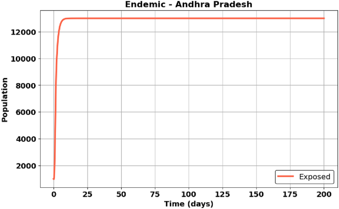
EE – Andhra Pradesh State – Exposed population (E).
Fig. 30 
EE – Maharashtra State – Exposed population (E).
Fig. 31 
EE – Tamil Nadu State – Exposed population (E).
Fig. 32 
EE – Andhra Pradesh State – Infected population (I).
Fig. 33 
EE – Maharashtra State – Infected population (I).
Fig. 34 
EE – Tamil Nadu State – Infected population (I).
Fig. 35 
EE – Andhra Pradesh State – Recovered population (R).
Fig. 36 
EE – Maharashtra State – Recovered population (R).
Fig. 37 
EE – Tamil Nadu State – Recovered population (R).
-
-
Figure 20, 21 and 22: Infected Population
-
Figure 20: Infected Population in Andhra Pradesh. The infected population ((I)) rises sharply, peaks early, and then declines as the disease is controlled through recovery.
-
Figure 21: Infected Population in Maharashtra. The infected population ((I)) peaks more dramatically, reflecting a faster spread of the disease.
-
Figure 22: Infected Population in Tamil Nadu. The infected population ((I)) peaks later, with a slower rise in infections.
-
-
Figure 23, 24 and 25: Recovered Population
-
Figure 23: Recovered Population in Andhra Pradesh. The recovered population ((R)) increases steadily as more individuals recover from the infection.
-
Figure 24: Recovered Population in Maharashtra. The recovered population ((R)) increases more quickly due to a higher initial infection rate, leading to faster recoveries.
-
Figure 25: Recovered Population in Tamil Nadu. The recovered population ((R)) increases steadily, similar to Andhra Pradesh, though at a slightly slower pace.
-
The following figures illustrate the dynamics of the (S), (E), (I), and (R) compartments during the endemic phase across Andhra Pradesh, Maharashtra, and Tamil Nadu.
-
Figures 26, 27 and 28: Susceptible Population
-
Figure 26: In Andhra Pradesh, the susceptible population decreases steadily, reflecting prolonged exposure during the endemic phase.
-
Figure 27: Maharashtra shows a more rapid decline in the susceptible population due to higher interaction rates.
-
Figure 28: Tamil Nadu exhibits a gradual decrease in the susceptible population over time.
-
-
Figures 29, 30 and 31: Exposed Population
-
Figure 29: Andhra Pradesh shows an initial rise and eventual stabilization of the exposed population as transmission stabilizes.
-
Figure 30: Maharashtra experiences a sharper increase in the exposed population, with a higher stabilization point.
-
Figure 31: Tamil Nadu demonstrates moderate growth and a plateau in the exposed population during the endemic phase.
-
-
Figures 32, 33 and 34: Infected Population
-
Figure 32: Andhra Pradesh sees a peak in the infected population, followed by a decline as recovery rates improve.
-
Figure 33: Maharashtra shows a higher peak in infections due to its population density and disease transmission rates.
-
Figure 34: Tamil Nadu’s infected population rises more gradually and peaks later, reflecting extended disease persistence.
-
-
Figures 35, 36 and 37: Recovered Population
-
Figure 35: Andhra Pradesh shows steady growth in the recovered population as individuals recover.
-
Figure 36: Maharashtra experiences rapid recovery, leading to a sharp increase in the recovered population.
-
Figure 37: Tamil Nadu exhibits consistent growth in the recovered population over time.
-
Conclusion
This study developed and analyzed a modified SEIR model to understand the dynamics of COVID-19 in three states of India-Andhra Pradesh, Maharashtra, and Tamil Nadu-using real data from May 2020. By incorporating region-specific epidemiological parameters and control strategies such as vaccination, mask-wearing, and social distancing, the model provides valuable insights into the progression and control of the pandemic.
Our study’s main innovation is the use of Pontryagin’s Maximum Principle (PMP) to optimise vaccination plans, guaranteeing the greatest possible decrease in infection rates while taking biological limitations like vaccine effectiveness, fading immunity, and reinfection risks into account. Furthermore, we examine the stability of Endemic Equilibrium (EE) and Disease-Free Equilibrium (DFE), providing information on the prerequisites for long-term COVID-19 persistence and eradication. The impact of important biological parameters is further revealed by sensitivity analysis, which highlights how vaccination can shorten the duration of an infection and lower its potential for transmission. Our study connects theoretical modelling with realistic, biologically based public health policies by including real-world epidemiological data, increasing its applicability to healthcare practitioners and policymakers.
Summary of findings
Basic Reproduction Number ((R_0)):
-
Tamil Nadu: (R_0 = 0.0334)
-
Maharashtra: (R_0 = 0.2170)
-
Andhra Pradesh: (R_0 = 0.1930)
These values indicate varying levels of transmissibility, with Maharashtra having the highest potential for disease spread. Tamil Nadu, with the lowest (R_0), reflects a relatively controlled transmission rate, possibly due to effective policy enforcement and public compliance.
Endemic Equilibrium ((S^*), (E^*), (I^*), (R^*)):
-
Tamil Nadu: (S^* = 5390, E^* = 14750, I^* = 73209, R^* = 2584916)
-
Maharashtra: (S^* = 3229, E^* = 30219, I^* = 150600, R^* = 4026424)
-
Andhra Pradesh: (S^* = 1152, E^* = 13682, I^* = 68153, R^* = 1894890)
Maharashtra has the highest infectious population ((I^* = 150600)), signifying a greater burden on healthcare systems, while Andhra Pradesh and Tamil Nadu exhibit lower endemic infection levels.
Role of sensitivity analysis
Sensitivity analysis identifies parameters with the most significant impact on (R_0):
-
Transmission Rate ((beta)): Positive sensitivity ((E_beta = 1.000) for all states) highlights its critical role in driving disease spread.
-
Progression ((sigma)) and Recovery ((phi)): Negative indices ((-0.286) and (-0.714), respectively) indicate their importance in reducing (R_0).
Maharashtra and Andhra Pradesh share similar sensitivity patterns, while Tamil Nadu shows slightly better control of transmission dynamics due to its lower sensitivity to mortality ((gamma)).
Analysis of optimal control strategy ((M))
The graphs illustrate the impact of vaccine administration ((M)) on susceptible ((S)), exposed ((E)), infectious ((I)), and recovered ((R)) populations across the three states. The following insights emerge:
Tamil Nadu:
-
Better Reduction in (I): Tamil Nadu shows a sharper decline in (I) at higher (M) values, reflecting efficient vaccination campaigns.
-
Rapid Recovery ((R)): The recovered population ((R)) increases steadily with (M), achieving stability faster than other states.
Maharashtra:
-
Highest Initial Burden: With the largest infectious population ((I_0 = 150600)), Maharashtra experiences a slower decline in (I) even as (M) increases.
-
Delayed Stability: The state requires higher (M) values and more time to reach equilibrium compared to Tamil Nadu and Andhra Pradesh.
Andhra Pradesh:
-
Moderate Decline in (I): While the decline in (I) is evident, it is less pronounced than in Tamil Nadu due to a higher initial susceptible population ((S_0 = 25000)).
-
Slower Recovery ((R)): The recovered population increases more gradually, indicating room for improvement in vaccine rollout and policy implementation.
Comparative assessment of control strategy implementation
Based on the analysis, Tamil Nadu emerges as the state with the most effective implementation of control strategies. The key reasons include:
-
1.
Lowest (R_0) Value: Tamil Nadu’s (R_0 = 0.0334) suggests effective policy enforcement, such as mask mandates and vaccination campaigns.
-
2.
Rapid Reduction in (I): The infectious population declines faster in Tamil Nadu, reflecting the success of targeted interventions.
-
3.
Quicker Stability in (R): Tamil Nadu achieves a stable recovered population earlier, reducing the overall burden on healthcare systems.
Maharashtra, despite higher infection rates, benefits significantly from vaccination but requires more aggressive implementation of control measures. Andhra Pradesh shows moderate progress but could further enhance its strategies to achieve faster recovery.
Policy implications
-
Strengthen Vaccination Programs: Increasing (M) values universally reduces (I) and boosts (R). States should prioritize higher vaccine coverage to achieve endemic stability.
-
Region-Specific Interventions:
-
Maharashtra requires urgent measures to address its higher infectious population and slower recovery rates.
-
Andhra Pradesh should focus on reducing its large initial susceptible population.
-
-
Integrated Measures: Combining vaccination with other controls, such as quarantine and public awareness, can amplify the benefits of (M).
Final conclusion
This study demonstrates the effectiveness of the SEIR model in analyzing COVID-19 dynamics and designing optimal control strategies. Key takeaways include:
-
1.
Tamil Nadu outperforms Maharashtra and Andhra Pradesh in implementing vaccination and other control measures.
-
2.
Sensitivity analysis highlights the importance of managing transmission ((beta)), progression ((sigma)), and recovery ((phi)) rates to control (R_0).
-
3.
Optimal control strategies, particularly vaccine administration ((M)), significantly reduce the burden of the infectious population and increase recovery rates.
The model’s applicability to real datasets was demonstrated through numerical simulations that closely matched the reported data for each state. Critical parameters such as the reproduction number ((R_0)), infection progression rates, and recovery rates were derived and validated against observed data trends. For all three states, the calculated reproduction numbers were significantly influenced by control strategies, such as vaccination rates and compliance with public health measures, showcasing the effectiveness of these interventions in reducing the spread of infection.
The sensitivity analysis identified key parameters that have the most significant impact on (R_0). The results emphasize that increasing the transmission reduction measures (e.g., mask usage, social distancing) and vaccination efforts leads to a drastic decrease in the infection spread. Optimal control strategies, when implemented, were shown to flatten the infection curve in the simulations, highlighting the potential for real-world application of these strategies. Specifically, Maharashtra demonstrated the highest (R_0), indicating a greater initial infection risk, whereas Tamil Nadu showed a more gradual response to control interventions. Andhra Pradesh, on the other hand, exhibited moderate infection dynamics but benefited significantly from the implementation of control measures.
The future implications of this model are highly promising. The framework can be extended by incorporating additional real-time data and new control strategies, such as improved contact tracing, targeted lockdowns, and early isolation of infectious individuals. These enhancements would further strengthen the model’s predictive capability and its utility for public health decision-making. By dynamically adjusting control parameters based on real-time infection data, policymakers can optimize resource allocation and achieve a significant reduction in infection rates and a faster recovery for the population.
In conclusion, the proposed SEIR model not only validates the current control measures but also provides a flexible and robust framework that can adapt to future scenarios. Its ability to integrate new strategies, such as increased vaccination coverage or novel therapeutics, ensures its continued relevance in mitigating the spread of infectious diseases. If applied systematically across all three states and expanded to other regions, this model has the potential to drastically reduce the burden of infection and accelerate recovery, contributing to better public health outcomes during pandemics.


Responses