Stabilization of Kerr-cat qubits with quantum circuit refrigerator

Introduction
In the quantum regime, where the nonlinearity is greater than the photon loss rate, a periodically driven superconducting nonlinear resonator can operate as a Kerr-cat qubit, providing a promising route to a quantum computer1,2,3,4,5. For example, a Kerr-cat qubit can be implemented by a parametrically-driven superconducting resonator with the Kerr nonlinearity, Kerr parametric oscillator (KPO)6,7,8, and a superconducting nonlinear asymmetric inductive element (SNAIL)9,10. Two meta-stable states of the driven superconducting resonators are utilized as a Kerr-cat qubit. Because of their long lifetime, the bit-flip error is much smaller than the phase-flip error. This biased nature of errors enables us to perform quantum error corrections with less overhead compared to other qubits with unbiased errors11,12. Qubit-gate operations have been intensely studied4,5,13,14,15,16,17 and demonstrated9,18, and high error-correction performance by concatenating the XZZX surface code12 with Kerr-cat qubits19 was examined. Kerr-cat qubits also find applications to quantum annealing4,20,21,22,23,24,25,26,27 and Boltzmann sampling28, and offer a platform to study quantum phase transitions29,30,31 and quantum chaos1,32,33.
Kerr-cat qubits are vulnerable to pure dephasing of the resonator, which causes excitations outside the qubit subspace. Such leakage errors into excited states are hard to correct by quantum error-correction protocols, which only deal with errors in the qubit subspace. Although engineered two-photon loss realized with the help of a dissipative mode13,34 and frequency-selective dissipation35 can mitigate unwanted excitations, no experimental demonstration with a KPO or a SNAIL has been reported. On the other hand, external single-photon loss in the resonator can reduce the excitations by transferring the population from excited states to the qubit subspace, but it generates phase-flips of the Kerr-cat qubit (errors in the qubit subspace)21. Therefore, the photon loss rate needs to be small while still being large enough to mitigate the effects of pure dephasing. Since it is difficult to determine the amplitude of the pure dephasing before measurement, and the amplitude depends on the parameters used for an operation of the Kerr-cat qubit, making the photon loss tunable is a solution to meet the above requirement.
The electron tunneling through a microscopic junction can occur accompanied by energy exchange with the environment36,37,38,39,40. Thus, controlled electron tunneling offers a way to selectively cool or heat devices in a cryogenic refrigerator41. Remarkably, on-chip refrigeration of a superconducting resonator, which is based on the photon-assisted electron tunneling through normal metal–insulator–superconductor (NIS) junctions, was demonstrated42,43. This device, called a quantum circuit refrigerator (QCR), can operate as a tunable source of dissipation for quantum-electric devices such as qubits44,45,46,47. More recently, the qubit reset with QCR was demonstrated48,49. While several works on the effect of the QCR on linear resonators, two-level systems and transmons have been reported, it remains largely unexplored for periodically driven systems such as KPOs. Although it is intuitively expected that the QCR can cool KPOs more or less, it is nontrivial how the following characteristics of KPOs affect the effectiveness of the QCR: (i) the system is periodically driven, and its effective energy eigenstates exist in a rotating frame; (ii) the system typically has degenerate energy eigenstates with the biased errors. Another important question is whether the biased nature of errors of KPOs will be preserved under the operation of the QCR.
We study the effect of electron tunneling through microscopic junctions on a periodically driven superconducting resonator, particularly considering a superconductor–insulator–normal metal–insulator–superconductor (SINIS) junction coupled to a KPO. We develop the master equation that can describe the effect of the electron tunnelings on the coherence of the KPO as well as the inter-level population transfers. The performance of the cooling based on the QCR is examined with the master equation. We also study drawbacks of the QCR such as the QCR-induced phase flip and bit flip. We show that the QCR-induced bit flip is suppressed by more than six orders of magnitude when relevant energy levels of the KPO degenerate due to quantum interference of the tunneling processes, and thus, the biased nature of errors is preserved.
Although our theory can be applied to a broader class of superconducting circuits, we particularly consider a KPO coupled to a SINIS junction of which the schematic is shown in Fig. 1A. When the SINIS junction is biased by a voltage VB, the tunneling of quasiparticles occurs through the junctions. The normal metal island of the SINIS junction is capacitively coupled to the KPO. The quasiparticle tunneling causes the change in the electric charge of the normal metal island and influences the KPO via the aforementioned capacitive coupling. The interaction between quasiparticles and the KPO mediated by the normal metal island can cause transitions between energy levels of the KPO accompanied by the quasiparticle tunneling. A tunneling quasiparticle can absorb energy from the KPO. Such quasiparticle tunneling is sometimes called photon-assisted tunneling36. The bias voltage can be used to control the rate of deexcitations (cooling) and excitations (heating) of the KPO. Figure 1B shows the energy diagram for single-quasiparticle tunneling corresponding to a bias voltage where the photon-assisted quasiparticle tunneling is observed. By absorbing energy from the KPO, a quasiparticle can tunnel to an unoccupied higher-energy state on the opposite side of the junction.

A Schematic of the SINIS junction coupled to the KPO. VB is the bias voltage applied to the SINIS junction. Cc is the coupling capacitance. The arrows indicate quasiparticle tunnelings. B Energy diagram for the single-quasiparticle tunneling at a bias voltage VB < 2Δ/e. The black solid curves at the normal metal and the superconductors represent the Fermi-Dirac distribution function and the density of states in the superconductors, respectively. The colored and shaded areas represent the occupied and unoccupied states, respectively. The straight arrows indicate the quasiparticle tunnelings from an initial energy state (beginning of the arrow) to a final energy state (end of the arrow). The wavy arrows indicate energy absorption from the KPO. C Effective circuit of the system composed of a NIS junction, the KPO, and the coupling capacitance Cc. The part in orange is the normal-metal island of the NIS junction with q excess quasiparticles, and the part shaded by light blue is the KPO formed with capacitance C and a SQUID with the Josephson energy EJ and an external magnetic flux Φex(t). The circuit has only one of the NIS junctions with the junction capacitance Cj and the tunneling resistance RT. Cm is the capacitance of the metallic island to the ground, which includes the capacitance of another junction. V = VB/2 is the bias voltage applied to a single NIS junction. D Energy diagram of the KPO. The horizontal solid and dashed lines represent even and odd parity energy eigenstates, respectively. The two lowest degenerate levels shaded by light blue are qubit states. The red arrows indicate excitations induced by the pure dephasing. The blue solid (dashed) arrows indicate deexcitations by the QCR to opposite (the same) parity energy levels. E Bloch sphere of the Kerr-cat qubit. Schematic drawings of the Wigner functions corresponding to the eigenstates of X, Y, and Z Pauli operators and excited states outside the qubit subspace are presented.
Figure 1C is the effective circuit of the system used to discuss the effect of one of the NIS junctions. Another junction is regarded as a capacitor, in which capacitance is included in the capacitance of the metallic island to the ground44. The SQUID of the KPO is subjected to an oscillating magnetic flux with the angular frequency ωp7. Cc is the coupling capacitance between the normal-metal island and the KPO. The effective Hamiltonian of the KPO is written, in a rotating frame at ωp/2, as
where ΔKPO, χ, and β are the detuning, the Kerr nonlinearity, and the amplitude of the pump field, respectively (see, e.g., ref. 7 and subsection “Unitary transformations” in the Methods section for the derivations and the definitions of the parameters). In this paper, we consider the case that ΔKPO = 0. The schematic energy diagram of the KPO is sketched in Fig. 1D, where the order of the energy levels is determined by the energy in the lab frame, and is opposite to that in the rotating frame. The two lowest energy levels are degenerate and written as
with coherent states (leftvert pm alpha rightrangle), where (alpha =sqrt{2beta /chi }) and ({N}_{pm }={(2pm 2{e}^{-2{alpha }^{2}})}^{-1/2}). These states define a Kerr-cat qubit. Because of their degeneracy and orthogonality, (leftvert {phi }_{pm alpha }rightrangle =(leftvert {phi }_{0}rightrangle pm leftvert {phi }_{1}rightrangle )/sqrt{2}) are also energy eigenstates orthogonal to each other. We have (leftvert {phi }_{pm alpha }rightrangle simeq leftvert pm alpha rightrangle) for sufficiently large α. We work on a basis in which (leftvert {phi }_{pm alpha }rightrangle) are along the z-axis of the Bloch sphere [Fig. 1E]. Because ({H}_{{rm{KPO}}}^{({rm{RF}})}) conserves parity, its linearly independent eigenstates can be taken so that they have either even or odd parity. We represent energy eigenstates with even and odd parity as (leftvert {phi }_{2n}rightrangle) and (leftvert {phi }_{2n+1}rightrangle), respectively, where n(≥0) is an integer.
As experimentally observed in ref. 27 and shown numerically in subsection “Pure dephasing and single-photon loss” in the Methods section, the pure dephasing of the KPO causes transitions from (vert {phi }_{0,1}rangle) to excited states with the same parity [Fig. 1D]. The role of the QCR is to bring the population of the states back to the qubit subspace by absorbing excess energy from the KPO. The main purpose of this paper is to present the cooling performance of the QCR and possible drawbacks such as QCR-induced phase flip (transition between (leftvert {phi }_{0}rightrangle) and (leftvert {phi }_{1}rightrangle)) and bit flip (transition between (vert {phi }_{alpha }rangle) and (vert {phi }_{-alpha }rangle)).
Results
Master equation and rate of QCR-induced transitions
The Hamiltonian of the system composed of quasiparticles in a NIS junction and the effective circuit in Fig. 1C is written as
where HQP is the Hamiltonian of quasiparticles given by
Here, e is the elementary charge, and subscript QP indicates quasiparticle. ckσ and dlσ are the annihilation operators for quasiparticles in the superconducting electrode and the normal-metal island, respectively. εk and εl are the energies of quasiparticles with wave numbers k and l, while σ denotes their spins. In our model, quasiparticles in the superconducting electrodes are treated as quasiparticles in the normal-metal island except that the density of states is different (the semiconductor model)50,51. The energy shift of −eV in the first term represents the effect of the bias voltage V = VB/2. Tunneling Hamiltonian HT represents the tunneling of quasiparticles and the interaction between quasiparticles and the superconducting circuit, and is written as44
where φN is a dimensionless flux, that is, ℏφN/e is the flux, ΦN, defined by time integration of the node voltage. The factor ({e}^{-i{varphi }_{N}}) represents the shift of the electric charge in the normal-metal island accompanied by quasiparticle tunneling. The Hamiltonian of the effective circuit is written as
where CN = Cc + Cm + Cj, ({C}_{r}=C+{alpha }_{c}{{C}_{Sigma }}_{m}), αc = Cc/CN, ({{C}_{Sigma }}_{m}={C}_{m}+{C}_{j}), Qj = CjV, and QN is the conjugate charge of the flux at the normal-metal island ΦN (see ref. 44 for the derivation of the Hamiltonian of a similar circuit). Φ is the flux at the KPO, and Q is its conjugate charge. We have the commutation relations, [Φ, Q] = [ΦN, QN] = iℏ. We assume that the Josephson energy EJ(t) is modulated as ({E}_{J}(t)={E}_{J}+delta {E}_{J}cos ({omega }_{p}t)) via a time-dependent magnetic flux in the SQUID (see subsection “Unitary transformations” in the Methods section).
For later convenience and for moving into the rotating frame at frequency ωRF = ωp/2, we apply unitary transformations, by which HT and H0 are transformed to ({H}_{T}^{({rm{RF}})}) and ({H}_{0}^{({rm{RF}})}) while HQP is unchanged (see subsection “Unitary transformations” in the Methods section for details). In the rotating-wave approximation, ({H}_{0}^{({rm{RF}})}) is written as
where ({Q}_{N}leftvert qrightrangle =eqleftvert qrightrangle), and q is an integer denoting the excess charge number in the normal-metal island. On the other hand, ({H}_{T}^{({rm{RF}})}) can be written as
where (leftvert mrightrangle) denotes a Fock state of the KPO. The first and second indices of (vert q,mrangle (=vert qrangle otimes vert mrangle )) denote the state of the normal-metal island and the KPO, respectively. We will regard ({H}_{T}^{({rm{RF}})}(t)) as a perturbation in the derivation of the master equation for the KPO.
Suppose that (vert {psi }_{mu ({mu }^{{prime} })}rangle) is an eigenstate of (H={H}_{{rm{QP}}}+{H}_{0}^{({rm{RF}})}) with energy ({E}_{mu ({mu }^{{prime} })}), and we have
We divide the system into two parts: the KPO and the others, that is, quasiparticles and the normal-metal island. The latter is called the environment. An eigenstate of H can be expressed as (vert {psi }_{mu }rangle =vert {phi }_{mu },{{mathcal{E}}}_{mu }rangle (=vert {phi }_{mu }rangle otimes vert {{mathcal{E}}}_{mu }rangle )), where (vert {phi }_{mu }rangle) is an eigenstate of ({H}_{{rm{KPO}}}^{({rm{RF}})}) with energy ({E}_{{phi }_{mu }}) and (vert {{mathcal{E}}}_{mu }rangle) denotes a state of the environment with energy ({E}_{{{mathcal{E}}}_{mu }}). The reduced density matrix for the KPO is obtained by tracing out the environment and is written as
with the density matrix of the total system ρ(t) and the matrix elements given by
We can derive the master equation for the KPO by tracing out the environment from the equation of motion for the total system and also by taking into account the effect of another NIS junction (see subsection “Derivation of the master equation” in the Methods section for the derivation). The master equation is written as
where ({omega }_{{phi }_{mu },{phi }_{{mu }^{{prime} }}}=({E}_{{phi }_{mu }}-{E}_{{phi }_{{mu }^{{prime} }}})/hslash), and
and ns is the density of states of the quasiparticles in the superconducting electrode given by
with the superconductor gap parameter Δ and the Dynes parameter γD52. The Fermi-Dirac distribution function is defined by (f(E,T)=1/[{e}^{E/({k}_{B}T)}+1]) with kB the Boltzmann constant, and TN and TS the electron temperature at the normal-metal island and the superconducting electrodes, respectively. The probability, denoted by pq, that the state of the normal-metal island is (leftvert qrightrangle), is determined using the elastic tunneling of quasiparticles, in which quasiparticles do not exchange energy with the KPO (see subsection “Probability pq” in the Methods section). In Eq. (13), (mathop{sum }nolimits_{{phi }_{{nu }^{{prime} }}}^{{prime} }), (mathop{sum }nolimits_{{phi }_{xi }}^{{prime} }), and (mathop{sum }nolimits_{{phi }_{xi }}^{{primeprime} }), respectively, denote the summation with respect to the state of the KPO, ({phi }_{{nu }^{{prime} }}), ϕξ, and ϕξ, which satisfy
And, ({eta }_{{phi }_{mu },{phi }_{nu }}^{(f,delta m)}) and ({eta }_{{phi }_{mu },{phi }_{nu }}^{(b,delta m)}) are defined by
while ({varepsilon }_{l}^{(f,delta m,i)}) and ({varepsilon }_{l}^{(b,delta m,i)}) for i = 1, 2, 3 are defined by
Here, EN = e2/(2CN). In Eq. (16), ρc is the interaction parameter defined by ({rho }_{c}={alpha }_{c}^{2}sqrt{{E}_{C}/(8{E}_{J})}) with EC = e2/(2Cr). The translation operator D(X) is defined as (D(X)=exp [X{a}^{dagger }-{X}^{* }a]). (langle {m}^{{prime} }| D(i{rho }_{c}^{frac{1}{2}})| mrangle) is given as53
where (l=m-{m}^{{prime} }), and ({L}_{m}^{l}) is the generalized Laguerre polynomials. The superscript f of ({eta }_{{phi }_{mu },{phi }_{nu }}) and εl denotes the forward tunneling where the number of quasiparticles increases in the normal-metal island, while b denotes opposite (backward) tunneling. Because of Eq. (12), Γ(1)(ϕi, ϕi, ϕj, ϕj, V) can be regarded as the rate of the transition from (| {phi }_{j}rangle) to (leftvert {phi }_{i}rightrangle) caused by the QCR and is quantitatively studied in the following section. The other Γs are also important to describe the dynamics of the KPO.
Cooling performance of QCR
We quantitatively examine the cooling performance of the QCR which is controlled with the bias voltage V. The results presented in the figures below are obtained through numerical simulations. Figure 2A shows the voltage dependence of the dominant transition rates relevant to cooling, heating, and phase flip of the KPO for experimentally feasible parameters, while Fig. 2B shows the rates of other transitions to the qubit states. The transition rates from excited states to the qubit states (cooling rates) can be changed by more than four orders of magnitude for the used parameters. The cooling rates dominate over heating rates, especially for 30 GHz < eV/h < 50 GHz as shown in Fig. 2A. These results suggest that the QCR can serve as an on-chip refrigerator for the KPO reducing the population of excited states, and the cooling power can be tuned over a wide range by the bias voltage. The phase-flip rate also increases with V as do the cooling rates. We note that the results in Fig. 2A, B, D are the rates of the QCR-induced transitions. In our theory, these rates are independent of the transitions caused by other decoherence sources such as the single-photon loss and the pure dephasing, which are considered later.
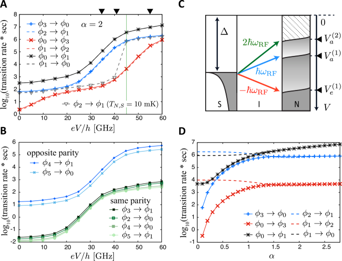
A Voltage dependence of the rates of dominant transitions corresponding to phase flip (black), cooling (blue), and heating (red) of the KPO for α = 2. The parameters used are ρc = 5 × 10⁻⁵, χ/2π = 10 MHz, ωc/2π = 7 GHz, Δ = 200 μeV, ΔKPO/2π = 0 MHz, RT = 50 kΩ, γD = 10−4, β/2π = 20 MHz, and TN,S = 100 mK. The values of the parameters, except for ρc, are comparable to the ones measured or used in the experiments27,42. The value of ρc is smaller than that used in the previous work44. The data points in gray color are for TN,S = 10 mK. The voltage indicated by the black triangles are ({V}_{a}^{(2)}), ({V}_{a}^{(1)}), and ({V}_{e}^{(1)}) in (C). The green vertical line indicates eV/h = 45 GHz used in (D). B The same things as (A) but for other transitions from excited states to the qubit states. C Schematic of energy diagram of a NIS junction. The dark green, light blue, and red arrows indicate two-photon-absorption, single-photon-absorption, and single-photon-emission processes, respectively. The minimum voltages at which these processes can occur are ({V}_{a}^{(2)}), ({V}_{a}^{(1)}), and ({V}_{e}^{(1)}) for TN,S = 0, respectively. We have (e{V}_{a}^{(2)}/hsimeq 34) GHz, (e{V}_{a}^{(1)}/hsimeq)41 GHz, and (e{V}_{e}^{(1)}/hsimeq)55 GHz for the parameters used. D α dependence of relevant transition rates for eV/h = 45 GHz. The color scheme is the same as in (A).
The bias voltage dependence of the transition rates can be understood from an energy diagram of a NIS junction for single-quasiparticle tunnelings [Fig. 2C], which also shows the minimum voltage at which each type of photon-assisted electron tunnelings can occur for TN,S = 0. The voltage is given by ({V}_{a}^{(2)}=(Delta -2hslash {omega }_{{rm{RF}}})/e), ({V}_{a}^{(1)}=(Delta -hslash {omega }_{{rm{RF}}})/e), and ({V}_{e}^{(1)}=(Delta +hslash {omega }_{{rm{RF}}})/e) for two-photon-absorption, single-photon-absorption, and single-photon-emission processes, respectively. The rate for transition (vert {phi }_{2}rangle to vert {phi }_{1}rangle) jumps at around (V={V}_{a}^{(1)}) for sufficiently low TN,S as seen in the result at TN,S = 10 mK in Fig. 2A. It suggests that this transition is due to the single-photon-absorption process. For the same reason, we consider that the opposite-parity (same-parity) transitions in Fig. 2A, B are caused mainly by a single-photon (two-photon) process. Note that two-photon-absorption processes can occur at a smaller voltage than the single-photon-absorption processes. On the other hand, with more experimentally feasible temperatures (TN,S = 100 mK), the increase of transition rates with respect to V is gradual and starts at smaller voltages than that for TN,S = 0. This is due to the temperature effect of the normal-metal island, which has a smooth variation of the Fermi distribution function. Figure 2D shows the α dependence of relevant transition rates for eV/h = 45 GHz. It is seen that the cooling and heating rates are insensitive to α for α > 1.5, which is in the typical parameter regime of the Kerr-cat qubit, and the cooling rates are two orders of magnitude higher than the heating rates. Therefore, the cooling effect is robust against changes in α. On the other hand, the phase-flip rate monotonically increases with α. We attribute this to the fact that the QCR approximately works as a source of single-photon loss with this bias voltage regime, and the single-photon loss causes the effective phase flip with the rate proportional to ∣α∣25. We also note that α = 0 corresponds to a transmon-type qubit, and the rate of the transition from (vert {phi }_{1}rangle) to (vert {phi }_{0}rangle) is the cooling rate for the transmon, while the rate of the transition from (vert {phi }_{0}rangle) to (vert {phi }_{1}rangle) is the heating rate.
Dynamics and stationary state of a KPO under operation of QCR
We study the dynamics and stationary states of the KPO under the operation of the QCR. We assume that, initially the QCR is off and the state of the KPO is (vert {phi }_{0}rangle). The QCR is turned on at t = tQCR as illustrated in Fig. 3A. We take into account the pure dephasing γp and the single-photon loss κ of the KPO which are not derived from the QCR, by including the second and the third terms of Eq. (35) in our equation of motion in addition to the effect of the QCR represented by Eq. (12) (see subsection “Pure dephasing and single-photon loss” in the Methods section). To distinguish the single-photon loss from the QCR-induced photon loss, we refer to it as the original single-photon loss. Relevant inter-level transitions for t < tQCR and t > tQCR are illustrated in Fig. 3A.
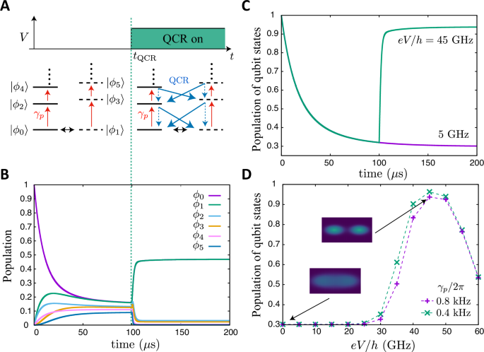
A Schedule of the QCR and relevant inter-level transitions when the QCR is off (left) and on (right). B Time dependence of the population of energy levels Pi and C the population of the qubit states P0 + P1, for κ/2π = 1.6 kHz and γp/2π = 0.8 kHz. The values of κ and γp are comparable to the ones measured for flux-tunable superconducting qubits58,59. D Population of the qubit states of the stationary state as a function of V for κ = 2γp. Insets are the Husimi Q function of the stationary states for γp/2π = 0.8 kHz. The other parameters used are the same as in Fig. 2.
Figure 3B shows the time dependence of Pi, the population of (leftvert {phi }_{i}rightrangle). For t < tQCR, Pi(>0) increases with time while P0 decreases. (We numerically integrated the equation of motion using a fourth-order Runge-Kutta method in order to simulate the dynamics of the KPO.) The increase of P1 is due to the phase flip from (vert {phi }_{0}rangle) to (vert {phi }_{1}rangle), indicated by a black arrow in Fig. 3A, caused by the original single-photon loss. The increase of Pi(>1) is due to heating induced by the pure dephasing denoted by the red arrows. For t > tQCR, Pi(>1) decreases, and Pi(≤1) increases due to the cooling effect represented by blue arrows. For sufficiently large t, (vert {phi }_{0}rangle) and (vert {phi }_{1}rangle) are equally populated due to the phase flip. The population of the qubit states P0 + P1 increases at t = tQCR for eV/h = 45 GHz as shown in Fig. 3C, because of high QCR-induced cooling rates dominating over γp. An increase in P0 + P1 is not seen for eV/h = 5 GHz because κ and γp govern the dynamics of the KPO. In Fig. 3D the population of the qubit states for the stationary state is exhibited as a function of the bias voltage for two different γp with κ = 2γp. The population can be higher than 0.93 by tuning the bias voltage while it is ~0.3 when the QCR is off. The population for smaller γp becomes higher than for larger γp at eV/h = 35 GHz. This is because less cooling rate is sufficient to see the effectiveness of the QCR for smaller γp. In the small voltage regime eV/h ≤ 15 GHz, the QCR is effectively off, and the population is determined by the ratio γp/κ. On the other hand, for large voltage regime eV/h ≥ 55 GHz, QCR-induced transitions dominate the effect of γp and κ. Therefore, the population is insensitive to γp and κ.
Biased nature of noise is preserved under operation of QCR
So far, we studied the effect of the QCR especially on the population Pi, which is the diagonal element of the density matrix of the KPO ({rho }_{{phi }_{i},{phi }_{i}}^{{rm{KPO}}}). Now we study the effect of the QCR on the off-diagonal elements of the density matrix, and present that the biased nature of errors of the KPO is preserved even under operation of the QCR, that is, the bit-flip rate is much smaller than the phase-flip rate. In order to see the impact of the QCR on the off-diagonal elements, we assume that the initial state is (vert {phi }_{alpha }rangle propto vert {phi }_{0}rangle +vert {phi }_{1}rangle). If decoherence caused by the QCR significantly enhances the decay of the off-diagonal elements, ({rho }_{{phi }_{0},{phi }_{1}}^{{rm{KPO}}}) and ({rho }_{{phi }_{1},{phi }_{0}}^{{rm{KPO}}}), the KPO rapidly approaches the mixed state of (vert {phi }_{alpha }rangle) and (vert {phi }_{-alpha }rangle). This can be interpreted as the QCR enhances bit flips, and the biased nature of errors of the KPO is lost. Importantly, as shown below, such decoherence is suppressed when (vert {phi }_{0}rangle) and (vert {phi }_{1}rangle) are degenerate.
According to Eq. (12), the Γs relevant to the change in ({rho }_{{phi }_{0},{phi }_{1}}^{{rm{KPO}}}) are Γ(1)(ϕ0, ϕ1, ϕi, ϕj), Γ(2)(ϕ0, ϕ1, ϕi), and Γ(3)(ϕ0, ϕ1, ϕi). In Fig. 4A, we present four dominant ones much greater than the others, Γ(1)(ϕ0, ϕ1, ϕ0, ϕ1), Γ(1)(ϕ0, ϕ1, ϕ1, ϕ0), Γ(2)(ϕ0, ϕ1, ϕ0), and Γ(3)(ϕ0, ϕ1, ϕ1), where the first two are positive and increase the off-diagonal element while the latter two are negative and decrease the off-diagonal element as illustrated in Fig. 4B. Here, Γ(1)(ϕ0, ϕ1, ϕ1, ϕ0) is the effect of the quantum interference arising from the degeneracy of (leftvert {phi }_{0}rightrangle) and (leftvert {phi }_{1}rightrangle), and its role is to preserve the coherence of the KPO (see subsection “Quantum interference effect associated with the level degeneracy” in the Methods section for the definition of the interference effect). Although its amplitude is smaller than the other three, its impact on the bit-flip rate is remarkable. Figure 4C shows the bit-flip rate (transition rate from (leftvert {phi }_{alpha }rightrangle) to (leftvert {phi }_{-alpha }rightrangle)) as a function of α. We define the QCR-induced bit-flip rate as ({Gamma }_{{rm{b-flip}}}=mathop{lim }nolimits_{Delta tto 0}langle {phi }_{-alpha }| {rho }^{{rm{KPO}}}(Delta t)| {phi }_{-alpha }rangle /Delta t), where ρKPO(Δt) is calculated using Eq. (12) with ({rho }^{{rm{KPO}}}(0)=vert {phi }_{alpha }rangle langle {phi }_{alpha }vert). Here, ({phi }_{-alpha }propto vert {phi }_{0}rangle -vert {phi }_{1}rangle), and 〈ϕα∣ϕ−α〉 = 0. If we neglect the quantum interference between the degenerate levels, i.e., let Γ(1)(ϕ0, ϕ1, ϕ1, ϕ0) = 0 in Eq. (12), the bit-flip rate increases with α, and the phase-flip rate shown in Fig. 2D does not significantly dominate over the bit-flip rate, that is, the biased nature of errors is not preserved. On the other hand, if we use Γ(1)(ϕ0, ϕ1, ϕ1, ϕ0) given in Eq. (13), the bit-flip rate steeply decreases as α increases and scales similarly to the case of single-photon loss, that is, the bit-flip rate is proportional to ({alpha }^{2}{e}^{-4{alpha }^{2}}) (see subsection “Pure dephasing and single-photon loss” in the Methods section). Then, the bit-flip rate is much smaller than the phase-flip rate, and therefore the biased nature of errors is preserved under operation of the QCR.
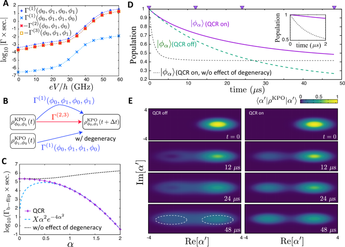
A Γs relevant to the change in ({rho }_{{phi }_{0},{phi }_{1}}^{{rm{KPO}}}) as a function of the voltage V applied to a NIS junction. The used parameters are the same as in Fig. 2. B Schematic of the role of the relevant Γs for the change of ({rho }_{{phi }_{0},{phi }_{1}}^{{rm{KPO}}}). Γ(2) and Γ(3) abbreviate Γ(2)(ϕ0, ϕ1, ϕ0) and Γ(3)(ϕ0, ϕ1, ϕ1), respectively. The blue (red) arrows indicate that positive (negative) Γs preserve (degrade) the coherence of the KPO. Γ(1)(ϕ0, ϕ1, ϕ1, ϕ0) is the effect of the quantum interference arising from the degeneracy between (leftvert {phi }_{0}rightrangle) and (leftvert {phi }_{1}rightrangle). C The QCR-induced bit-flip rate as a function of α. The black dotted curve represents the case where the QCR is on, but neglecting the quantum interference between the degenerate levels, that is, Γ(1)(ϕ0, ϕ1, ϕ1, ϕ0) = 0. The light-blue dashed line is the theory curve with the form of (propto {alpha }^{2}{e}^{-4{alpha }^{2}}). D Time dependence of the population of (leftvert {phi }_{alpha }rightrangle) when the QCR is on (purple solid curve) and when the QCR is off (green dashed curve), for κ/2π = 1.6 kHz and γp/2π = 0.8 kHz. The black thin dashed curve is for the case with Γ(1)(ϕ0, ϕ1, ϕ1, ϕ0) = 0. The triangles on the top of the figure indicate the time used in (E). E Husimi Q function, (langle {alpha }^{{prime} }| {rho }^{{rm{KPO}}}| {alpha }^{{prime} }rangle), at different times, for the case that the QCR is off (left) and on (right). We used eV/h = 40 GHz for (C–E).
We examine the stability of (leftvert {phi }_{alpha }rightrangle) under operation of the QCR by simulating the dynamics with the initial state of (leftvert {phi }_{alpha }rightrangle) and with eV/h = 40 GHz. We used a smaller bias voltage than in Fig. 3 to keep the QCR-induced phase-flip rate around 106 s−1 [see Fig. 2A]. The population of (leftvert {phi }_{alpha }rightrangle), denoted by Pα, is kept higher when the QCR is on than when the QCR is off as shown in Fig. 4D. It is noteworthy that if we neglect the quantum interference between the degenerate levels, Pα decreases even more rapidly than when the QCR is off. The population of qubit states is kept higher than 0.83 when the QCR is on due to the cooling effect, while it decreases approximately to 0.3 when the QCR is off as shown in Fig. 3D. Thus, the Kerr-cat qubit is stabilized by the energy absorption by the QCR and the quantum interference between the degenerate levels. Figure 4E shows the Husimi Q function, (langle {alpha }^{{prime} }| {rho }^{{rm{KPO}}}| {alpha }^{{prime} }rangle), at different times. The Q function widely spreads when the QCR is off because of the heating effect of the pure dephasing (see the result for t = 48 μs). On the other hand, it is confined around ({alpha }^{{prime} }=pm 2) when the QCR is on.
In general, interference can occur when the system (the KPO, in our case) has degenerate energy levels that are relevant to its dynamics, which do not have to be the ground states. It is also noteworthy that, even if such degenerate levels exist, the interference effect can be negligible depending on the properties of the energy eigenstates. The properties are reflected in the QCR-transition rates via ({eta }_{{phi }_{mu },{phi }_{nu }}^{f/b,delta m}). For example, in Fig. 4C, the difference between the QCR-induced bit-flip rates with and without the interference effect vanishes for α ≪ 1, where the pump amplitude becomes zero, and the form of the qubit Hamiltonian is the same as a transmon, while the two lowest levels, (leftvert 0rightrangle) and (leftvert 1rightrangle), are still degenerate in the rotating frame. It implies that the interference effect is negligible in this parameter regime.
Discussion
We have theoretically studied on-chip refrigeration for Kerr-cat qubits with a QCR. We have examined the QCR-induced deexcitations and excitations of a KPO by developing a master equation. The rate of the QCR-induced deexcitations can be controlled by more than four orders of magnitude by tuning the bias voltage across microscopic junctions. By examining the QCR-induced bit and phase flips, we have shown that the biased nature of errors of the qubit is preserved even under operation of QCR, that is, the bit-flip rate is much smaller than the phase-flip rate. We have found novel quantum interference in the tunneling process which occurs when the two lowest energy levels of the KPO are degenerate, and have revealed that the QCR-induced bit flip is suppressed by more than six orders of magnitude due to the quantum interference. Thus, QCR can serve as a tunable dissipation source that stabilizes Kerr-cat qubits, mitigating unwanted heating due to pure dephasing. Even though we particularly consider a KPO in this paper, our theory can be applied to more general superconducting circuits.
Although studying the performance of the QCR in specific applications of KPOs is beyond the scope of this paper, we comment on two possible applications and directions for future study. A possible application of the QCR is the stabilization of Kerr-cat qubits during gate-based quantum computing. The QCR can reduce leakage errors into excited states which cannot be corrected by quantum error-correction protocols that only deal with errors in the qubit subspace. The QCR may also find application in measurement-based state preparation of the Kerr-cat qubit, which was proposed in ref. 54 and experimentally utilized in refs. 55,56. Homodyne and heterodyne detections can be used to determine on which side of the effective double-well potential the KPO is trapped. Therefore, the measurement can tell us that the system is in either of (vert {phi }_{alpha }rangle) and (vert {phi }_{-alpha }rangle) if the system is confined in the qubit subspace because (vert {phi }_{alpha }rangle) and (vert {phi }_{-alpha }rangle) are in opposite potential wells. However, the total population of the excited states gives rise to the error of the state preparation. Because a QCR can reduce the population of excited states, activation of a QCR prior to the measurement-based state preparation would increase the fidelity of the state preparation.
We discuss the disadvantages of the use of a QCR. The relevant drawback of the QCR is the QCR-induced phase flip, which should be corrected for large-scale quantum computations. This limits the applicability of the QCR to cases where the pure dephasing rate is sufficiently smaller than the acceptable phase-flip rate, which will vary across different applications. The simple and wide tunability of the cooling rates of the QCR will help to adjust the cooling performance balanced against the unwanted QCR-induced phase flip. However, the use of a QCR will degrade system coherence to an impractical level for error correction when the pure dephasing rate is too high, although a QCR may still be useful for qubit reset. As shown in Fig. 2D, the QCR-induced phase-flip rate decreases as the size of coherent states α decreases. A possible way to mitigate the issue of the unwanted QCR-induced phase flip is to find an appropriate α that is small enough to achieve an acceptably slow QCR-induced phase-flip rate yet large enough to ensure practical biased noise.
As seen in Fig. 2A, there is a phase flip with the rate <103 s−1, even in the absence of the bias voltage V, due to finite photon-assisted electron tunneling. This residual phase flip can be reduced by decreasing the coupling strength between the QCR and the KPO, although this comes at the cost of reducing the maximum amplitude of the cooling rate. The heating rate at V = 0 is <10 s−1, and is therefore negligible.
We summarize the pros and cons of our scheme comparing it with the previous works based on two-photon dissipation13,34 and frequency-selective dissipation35. (i) Both of the previous schemes utilize additional resonators. In contrast, our scheme uses a SINIS junction which is significantly smaller in size compared to the resonators. (ii) The frequency-selective dissipation does not require any additional drives. The two-photon dissipation is activated by a microwave applied to the additional resonator, while the QCR is driven by a DC bias voltage across the junction. (iii) The QCR is insensitive to parameters of the KPO, such as resonance frequency, nonlinearity parameter, and pump amplitude, which is a useful feature for scaling up the system. In contrast, the frequency of the microwave used for the two-photon dissipation depends on the resonance frequencies of both the qubit and the additional resonator. For the frequency-selective dissipation, the resonance frequencies of the additional resonators must be nearly identical, and these frequencies are determined by the parameters of the KPO. (iv) The QCR also functions for relatively small values of α, e.g., α = 2, where the frequency-selective dissipation tends to increase bit flip errors compared to the case without the dissipation mechanism35. (v) The advantage of the previous schemes is that phase flip is not enhanced in an ideal situation, whereas our scheme induces phase flip.
In this paper, we neglected the Johnson-Nyquist noise from the normal metal island of the QCR, while the electron temperature of the normal metal island was accounted for in the calculation of the QCR-induced transition rates via the Fermi-Dirac distribution function. Although the Johnson-Nyquist noise could potentially affect the properties of the attached resonator and qubit, such an effect has not yet been observed in previous QCR measurements42,43,47,48,49. We attribute this to the fact that the electron temperature of the normal metal island at the voltage used for cooling is lower than that at V = 0, due to the tunneling of high-energy electrons enhanced by the bias voltage41,42, and that the volume of the normal meal island is small, typically on the order of 0.01 μm342.
In our derivation of the QCR-induced transition rates, the normal metal island is set in a stationary state determined by elastic electron tunneling. This is based on assumptions that the dynamics of the normal metal island are governed by elastic electron tunneling, which is much faster than the photon-assisted electron tunneling for the parameters used, and thus the stationary state determined by the elastic electron tunneling provides a good approximation for the state of the normal metal island. In ref. 45, the authors studied the charge dynamics of the normal metal island under the operation of the QCR, and showed that the effect of the charge dynamics on the qubit reset is limited for typical parameters. They also clarified that when the size of the normal metal island is much smaller and enters in the quantum dot regime, the dynamics of the normal metal island becomes significant, leading to the emergence of different phenomena. Studying charge dynamics with our system will be an interesting direction for future research.
Methods
Unitary transformations
We apply unitary transformations Uj, U, and URF to simplify the Hamiltonian and to move into a rotating frame at a frequency of ωp/2. We begin with Uj defined by
which satisfies ({U}_{j}({Q}_{N}+{Q}_{j}){U}_{j}^{dagger }={Q}_{N}). The unitary transformation Uj simplifies H0 by eliminating Qj as
Because there is no ΦN in the Hamiltonian we can further rewrite it as
where q is an integer denoting the number of the excess charge in the normal-metal island, that is, eq is the charge in the normal-metal island. Note that Uj does not change HQP and HT.
Next, we perform a unitary transformation
to simplify H0 in Eq. (21) to
by eliminating αceq from the second term, where we used the fact that ({U}_{q}=exp [frac{i}{hslash }{alpha }_{c}eqPhi ]) translates the charge operator as ({U}_{q}(Q+{alpha }_{c}eq){U}_{q}^{dagger }=Q). The operator U changes HT while HQP is unchanged. The effect of U on HT is discussed later. We further rewrite H0 by using (phi =frac{2e}{hslash }Phi) and n = Q/2e as
where [ϕ, n] = i, and HKPO(t) is the Hamiltonian of the KPO defined by
We focus on the Hamiltonian of the KPO, HKPO. The magnetic flux Φ(t) in the SQUID is harmonically modulated around its mean value with a small amplitude. EJ(t) is represented as ({E}_{J}(t)={bar{E}}_{J}cos (pi Phi (t)/{Phi }_{0})) where ({bar{E}}_{J}) is constant. We assume that (Phi (t)={Phi }_{{rm{dc}}}-{delta }_{p}{Phi }_{0}cos ({omega }_{p}t)), where Φdc, and δp(≪1) are constant. Then, EJ(t) can be approximated as ({E}_{J}+delta {E}_{J}cos ({omega }_{p}t)), where ({E}_{J}={bar{E}}_{J}cos (pi {Phi }_{{rm{dc}}}/{Phi }_{0})) and (delta {E}_{J}={bar{E}}_{J}pi {delta }_{p}sin (pi {Phi }_{{rm{dc}}}/{Phi }_{0})) (see, e.g., section 4.1 of ref. 8). The Taylor expansion leads to
The quadratic time-independent part of the Hamiltonian (26) can be diagonalized by using relations n = −in0(a − a†) and ϕ = ϕ0(a + a†), where ({n}_{0}^{2}=sqrt{{E}_{J}/(32{E}_{C})}) and ({phi }_{0}^{2}=sqrt{2{E}_{C}/{E}_{J}}) are the zero-point fluctuations. Taking into account up to the 4th order of ϕ, we obtain
where we have defined the resonance frequency ({omega }_{c}^{(0)}=frac{1}{hslash }sqrt{8{E}_{C}{E}_{J}}), the Kerr nonlinearity χ = EC/ℏ, the parametric drive strength (beta ={omega }_{c}^{(0)}delta {E}_{J}/(8{E}_{J})). We neglect the last term in the square brakets because it is much smaller than the other terms ((chi beta ll {omega }_{c}^{(0)})). We also drop c-valued terms in the expression above and obtain
Now, we move into a rotating frame at the frequency ωp/2 by transforming the system with unitary operator
where ({I}_{N}={sum }_{q}leftvert qrightrangle leftlangle qrightvert). After the unitary transformation, the KPO Hamiltonian is written as
To obtain Eq. (1), we use the rotating-wave approximation, which is valid when (| {omega }_{c}^{(0)}-{omega }_{p}/2|), χ/12, and 2β are all much smaller than 2ωp. The detuning ΔKPO in Eq. (1) is given by ΔKPO = ωc − ωp/2, where ωc is the dressed resonator frequency defined by ({omega }_{c}={omega }_{c}^{(0)}-chi). The term proportional to (beta {a}^{dagger }acos ({omega }_{p}t)) in Eq. (30) is omitted in the rotating-wave approximation, and therefore the dressed resonator frequency is independent of β.
We consider the effect of U and URF on HT. The unitary operators transform HT as
In the above equation, we used the following fact. Because the unitary operator ({U}_{e}={e}^{ifrac{e}{hslash }{Phi }_{N}}) shifts the charge state as
we have
In the derivation of Eq. (32), we used
The second term in Eq. (31) corresponds to the electron tunneling from the normal-metal island to the superconducting electrode (note that the positive charge in the normal-metal island increases because of this transition). By using (delta m={m}^{{prime} }-m) in Eq. (31), we can obtain Eq. (8).
Pure dephasing and single-photon loss
We consider a KPO without a SINIS junction. The master equation of the KPO is given by
where ({mathcal{D}}[hat{O}]rho =2hat{O}rho {hat{O}}^{dagger }-{hat{O}}^{dagger }hat{O}rho -rho {hat{O}}^{dagger }hat{O})13. Here, κ and γp are the single-photon-loss rate and the pure-dephasing rate, respectively. We define the transition rate from (vert {psi }_{i}rangle) to (vert {psi }_{f}rangle) due to the pure dephasing as
where ({rho }_{i}=leftvert {psi }_{i}rightrangle leftlangle {psi }_{i}rightvert) and 〈ψf∣ψi〉 = 0.
We examine the transition rates from (leftvert {psi }_{i}rightrangle =leftvert {phi }_{alpha }rightrangle) to other states. The transition rates normalized by γp are presented for different final states in Fig. 5A. The bit-flip rate (transition from (vert {phi }_{alpha }rangle) to (vert {phi }_{-alpha }rangle)) is suppressed as α increases, and is explicitly written as
with (x=frac{1}{sqrt{2}}({N}_{+}+{N}_{-})) and (y=frac{1}{sqrt{2}}({N}_{+}-{N}_{-})). ({Gamma }_{p}^{{phi }_{alpha }to {phi }_{-alpha }}/{gamma }_{p}) in Eq. (37) is approximated by (2{alpha }^{2}{e}^{-4{alpha }^{2}}) for sufficiently large ∣α∣. The transition rates outside the qubit subspace become much larger than the bit-flip rate as α increases. Especially transition rates to the adjacent excited states (vert {phi }_{2,3}rangle) are higher than γp itself for α > 1.4.
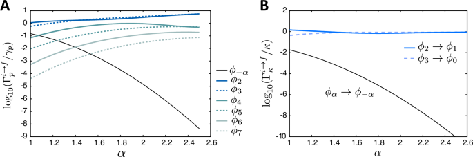
A Rate of transitions from (leftvert {phi }_{alpha }rightrangle) to other states due to the pure dephasing for ΔKPO = 0. The rate is normalized by γp. B Rate of deexcitations and bit flip caused by single-photon loss, where the rate is normalized by κ.
Similarly, we define the transition rate from (vert {psi }_{i}rangle) to (vert {psi }_{f}rangle) due to the single-photon loss as
Figure 5B shows the rate of relevant deexcitations to qubit states and bit flip caused by the single-photon loss. The bit-flip rate is suppressed as α increases, and is explicitly written as
which is well approximated by (2{alpha }^{2}{e}^{-4{alpha }^{2}}) for sufficiently large ∣α∣. The deexcitation rates asymptotically approach κ, that is, ({Gamma }_{kappa }^{{phi }_{0(1)}to {phi }_{3(2)}}to kappa), which is derived by using (vert {phi }_{2,3}rangle simeq frac{1}{sqrt{2}}(D(alpha )leftvert 1rightrangle mp D(-alpha )leftvert 1rightrangle )) for sufficiently large ∣α∣, where D(α) is the displacement operator defined by (D(alpha )=exp [alpha {a}^{dagger }-{alpha }^{* }a]).
Derivation of master equation
Suppose that at time t the state of the total system is given by
The time evolution of the total system is governed by the Schrödinger equation,
where ({V}_{mu nu }(t)=langle {psi }_{mu }| {H}_{T}^{({rm{RF}})}(t)| {psi }_{nu }rangle). Integrating Eq. (41) over time leads to the integral equation,
The validity of this equation can be easily confirmed by differentiating the equation with respect to time. Because of Eq. (42) we have
We use Eq. (43) on the right-hand side of Eq. (42) and repeat the same procedure to obtain the solution to second order in the perturbation as
As seen from Eq. (8), the perturbation can be written as ({V}_{mu nu }(t)={sum }_{delta m}{V}_{mu nu }^{(delta m)}exp [i{omega }_{{rm{RF}}}delta mt]) with ({V}_{mu nu }^{(delta m)}=langle {psi }_{mu }| {V}^{(delta m)}| {psi }_{nu }rangle), where
By using Eq. (44), we can write elements of the density matrix, ({a}_{mu }(t){a}_{{mu }^{{prime} }}^{* }(t)), as
The first term represents the evolution of the density matrix without the perturbation, the other terms represent the perturbation effects and include contributions from other elements of the density matrix. By using Eq. (46) and the results of subsection “Time integrals in Eq. (46)” in the Methods section, we obtain
where (mathop{sum }nolimits_{{phi }_{{nu }^{{prime} }}}^{{prime} }), (mathop{sum }nolimits_{{phi }_{xi }}^{{prime} }), and (mathop{sum }nolimits_{{phi }_{xi }}^{{primeprime} }), respectively, denote the summation with respect to ({phi }_{{nu }^{{prime} }}), ϕξ, and ϕξ which satisfies Eq. (15). Note that in Eq. (47), we have replaced the time interval t by Δt and shifted the origin of time by t.
The KPO master equation in Eq. (12) can be obtained by tracing out the environment from Eq. (47). The derivation is based on the following assumptions: At time t, the density matrix is represented as (rho (t)={rho }_{{rm{sys}}}(t)otimes {rho }_{{rm{env}}}^{(0)}). Here, ({rho }_{{rm{env}}}^{(0)}) is a thermal state of the environment written as ({rho }_{{rm{env}}}^{(0)}={sum }_{{mathcal{E}}}{p}_{{mathcal{E}}}leftvert {mathcal{E}}rightrangle leftlangle {mathcal{E}}rightvert) with energy eigenstates (leftvert {mathcal{E}}rightrangle), where ({p}_{{mathcal{E}}}) is the probability that the state of the environment is (leftvert {mathcal{E}}rightrangle). At time t + Δt, ρ(t + Δt) cannot be written as a product state of the system and the environment in general. We assume that the environment relaxes to the original state ({rho }_{{rm{env}}}^{(0)}) in time much shorter than Δt and the system can be represented again in a product state as (rho (t+Delta t)={rho }_{{rm{sys}}}(t+Delta t)otimes {rho }_{{rm{env}}}^{(0)}) where ({rho }_{{rm{sys}}}(t+Delta t)={{rm{Tr}}}_{{rm{env}}}rho (t+Delta t)). This process repeats at each time step Δt.
To obtain ({rho }_{{phi }_{mu },{phi }_{{mu }^{{prime} }}}^{{rm{KPO}}}(t+Delta t)) we calculate (sum_{{mathcal{E}}_{mu }}{a}_{mu }(t+Delta t){a}_{{mu }^{{prime} }}^{* }(t+Delta t)) using Eq. (47), where (vert {{mathcal{E}}}_{{mu }^{{prime} }}rangle =vert {{mathcal{E}}}_{mu }rangle). As an example, we consider the contribution of the term with ({a}_{nu }(t){a}_{{nu }^{{prime} }}^{* }(t)) in Eq. (47) particularly focusing on the term including ({c}_{ksigma }^{dagger }{d}_{lsigma }vert q+1,delta m+mrangle langle q,mvert) of V(δm) in Eq. (45). For deriving the contribution of the term to ({rho }_{{phi }_{mu },{phi }_{{mu }^{{prime} }}}^{{rm{KPO}}}(t+Delta t)), we note the following points: (a) we consider only the case where (leftvert {{mathcal{E}}}_{nu }rightrangle =leftvert {{mathcal{E}}}_{{nu }^{{prime} }}rightrangle) because ({a}_{nu }(t){a}_{{nu }^{{prime} }}^{* }(t)=0) otherwise; (b) the summation ∑k,l,σ is represented as 2∫ dεk∫ dεlns(εk), where ns is the density of state of the quasiparticles in the superconducting electrode; (c) summation ∑ν can be represented as ({sum }_{{{mathcal{E}}}_{nu }}{sum }_{{phi }_{nu }}), and summations ({sum }_{{mathcal{E}}_{mu }}{sum }_{{{mathcal{E}}}_{nu }}) are unified to ({sum }_{{{rm{QP}}}_{kl}}) which represents the sum running over the state of quasiparticles except for modes k and l because the state of modes k and l and the normal metal are determined by ({c}_{ksigma }^{dagger }{d}_{lsigma }vert q+1,delta m+mrangle langle q,mvert), while the states of other quasiparticle modes should be the same between (vert {{mathcal{E}}}_{mu }rangle) and (vert {{mathcal{E}}}_{nu }rangle); (d) ({sum }_{{{rm{QP}}}_{kl}}{a}_{nu }(t){a}_{{nu }^{{prime} }}(t)) leads to the factor ({p}_{q}[1-f({varepsilon }_{k},{T}_{S})]f({varepsilon }_{l},{T}_{N}){rho }_{{phi }_{nu },{phi }_{{nu }^{{prime} }}}^{{rm{KPO}}}(t)). Taking into account these points, we find that the contribution from ({rho }_{{phi }_{nu },{phi }_{{nu }^{{prime} }}}^{{rm{KPO}}}(t)) to ({rho }_{{phi }_{mu },{phi }_{{mu }^{{prime} }}}^{{rm{KPO}}}(t+Delta t)) is written as
The contributions from the other terms and another NIS junction to ({rho }_{{phi }_{mu },{phi }_{{mu }^{{prime} }}}^{{rm{KPO}}}(t+Delta t)) can be calculated in the same manner, and thus Eq. (12) is obtained. In Eq. (13), we replaced 4π∣T∣2/ℏ by 1/e2RT so that the tunnel resistance matches the measured one for a sufficiently large V50. The effects of the two NIS junctions are the same because they are identical in our model.
A comment on the derivation of the reduced master equation is in order. Although we considered a pure state in Eq. (41) when deriving the reduced master equation, the state at t should be regarded as a mixed state of such pure states. In our theory, the probability that the state of the system is each pure state is accounted for by factors such as pq and the Fermi-Dirac distribution function.
Time integrals in Eq. 46
We consider the time integrals in Eq. (46). First, we consider the integral
included in the fourth term of Eq. (46), where ω1 and ω2 are constant. ∣Y1(ω, t)∣ peaks at ω = ω1 and ω2. In this study, we consider the cases in which either ω1 = ω2 or two peaks are well separated.
When ω1 = ω2, the height of the peak is t2, while its width is of the order of 2π/t57. It is known that, for sufficiently large t, Y1 approaches a delta function, that is,
where E1 = ℏω1 = ℏω2. On the other hand, the integral can be neglected when two peaks are well separated because the height of the peaks is of the order of (sqrt{delta (E)}).
Next, we consider
included in the fifth and sixth terms in Eq. (46). ∣Y2(ω, t)∣ peaks at ω = ω1 and ω2. The integral can be neglected when two peaks are well separated because the height of the peaks is of the order of (sqrt{delta (E)}). When ω1 = ω2, Y2(ω, t) approaches a function represented by
where the imaginary part, ig, can be neglected because it is an odd function about E = E1 and the width becomes very narrow as t increases. By using these relations, we can obtain Eq. (47) from Eq. (46). The condition for two peaks to be considered sufficiently separated is that ∣ω1−ω2∣ is sufficiently larger than 2π/t because the width of each peak is of the order of 2π/t.
Note that the second term in Eq. (46) can be neglected for the following reasons. (vert {{mathcal{E}}}_{{mu }^{{prime} }}rangle) should be the same as (vert {{mathcal{E}}}_{{nu }^{{prime} }}rangle) so that the integral can contribute to the density matrix of the KPO, however if they are the same ({V}_{{mu }^{{prime} }{nu }^{{prime} }}^{(delta {m}^{{prime} })}=0) and thus the second term becomes zero. The third term can also be neglected for the same reason.
Probability p
q
Here, we follow the same method as ref. 44 to calculate pq, which defines the probability of the normal-metal island state being (leftvert qrightrangle). Because the elastic-tunneling rate is much larger than inelastic ones44, we assume that pq can be determined by the elastic-tunneling independently of the KPO state.
The population is written as
where Z is the normalization factor, and ({Gamma }_{q,m,m}^{pm }(V)) is defined by
with ({E}_{q}^{pm }=frac{{e}^{2}}{2{C}_{N}}(1pm 2q)), RK = h/e2, and
In Eq. (54), ({M}_{m,m}^{2}) is defined by
where ({L}_{m}^{l}({rho }_{c})) is the generalized Laguerre polynomials. We also have p0 = 1/Z and p−q = pq. Equivalently pq is written as
Quantum interference effect associated with the level degeneracy
We explain the concept of the interference effect associated with the level degeneracy, with particular focus on the integrand of the time integrals in the third line of Eq. (46),
where we replaced the second integral variable s with ({s}^{{prime} }) to distinguish it from the first. The contribution of this integrand to ({a}_{mu }(t){a}_{{mu }^{{prime} }}^{* }(t)) is schematically illustrated in Fig. 6A. The integrand can also be represented by the left pair of lines in Fig. 6B, as we consider the case where (vert {{mathcal{E}}}_{mu }rangle =vert {{mathcal{E}}}_{{mu }^{{prime} }}rangle) and (leftvert {{mathcal{E}}}_{nu }rightrangle =leftvert {{mathcal{E}}}_{{nu }^{{prime} }}rightrangle) in the calculation of the reduced density matrix for the KPO, as explained in the paragraph containing Eq. (10). This integrand can also be interpreted as the contribution from ({rho }_{{phi }_{nu },{phi }_{{nu }^{{prime} }}}^{{rm{KPO}}}(0)) to ({rho }_{{phi }_{mu },{phi }_{{mu }^{{prime} }}}^{{rm{KPO}}}(t)), because ({a}_{nu }(0){a}_{{nu }^{{prime} }}^{* }(0)) and ({a}_{mu }(t){a}_{{mu }^{{prime} }}^{* }(t)) are related to ({rho }_{{phi }_{nu },{phi }_{{nu }^{{prime} }}}^{{rm{KPO}}}(0)) and ({rho }_{{phi }_{mu },{phi }_{{mu }^{{prime} }}}^{{rm{KPO}}}(t)), respectively. The property of the time integral imposes a condition on the KPO states ({vert {phi }_{nu }rangle ,vert {phi }_{{nu }^{{prime} }}rangle }), as represented by the first line of Eq. (15). When there is a level of degeneracy, multiple sets of such initial states exist, each with different KPO states ({vert {phi }_{nu }rangle ,vert {phi }_{{nu }^{{prime} }}rangle }) that satisfy Eq. (15), but with the same environment states. We refer to the contributions from such initial states, with different KPO states ({vert {phi }_{nu }rangle ,vert {phi }_{{nu }^{{prime} }}rangle }) but the same environment states, as the quantum interference effect in this paper. Note that we term this contribution “quantum interference” when the initial environment states are identical as in Fig. 6B. The contributions should not be called “quantum interference” when the initial environment states are different, since there is no coherence between the different environment states.
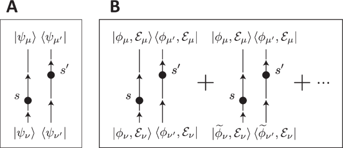
A Schematic of the contribution from the integrand in Eq. (58) to ({a}_{mu }(t){a}_{{mu }^{{prime} }}(t)). The left line represents ({V}_{mu nu }^{(delta m)}{e}^{i({omega }_{mu nu }+{omega }_{{rm{RF}}}delta m)s}{a}_{nu }(0)), while the right represents ({({V}_{{mu }^{{prime} }{nu }^{{prime} }}^{(delta {m}^{{prime} })})}^{* }{e}^{-i({omega }_{{mu }^{{prime} }{nu }^{{prime} }}+{omega }_{{rm{RF}}}delta {m}^{{prime} }){s}^{{prime} }}{a}_{{nu }^{{prime} }}^{* }(0)). B The left pair of the lines is the same thing as (A), where we used (leftvert {psi }_{mu }rightrangle =leftvert {phi }_{mu },{{mathcal{E}}}_{mu }rightrangle), and ({{mathcal{E}}}_{mu }={{mathcal{E}}}_{{mu }^{{prime} }}) and ({{mathcal{E}}}_{nu }={{mathcal{E}}}_{{nu }^{{prime} }}). The right pair is associated with the same environment states as the left, but different KPO states at t = 0, (leftvert {widetilde{phi }}_{nu }rightrangle) and (leftvert {widetilde{phi }}_{{nu }^{{prime} }}rightrangle). The KPO states corresponding to both the left and right pairs satisfy the first equation in Eq. (15).
This integrand is associated with ({Gamma }^{(1)}({phi }_{mu },{phi }_{{mu }^{{prime} }},{phi }_{nu },{phi }_{{nu }^{{prime} }},V)) in Eq. (13). The master equation in Eq. (12) accounts for the quantum interference via the summation with respect to the state of the KPO, ({phi }_{{nu }^{{prime} }}), which satisfies Eq. (15). As a result, it not only ({rho }_{{phi }_{0},{phi }_{1}}^{{rm{KPO}}}(0)) but also ({rho }_{{phi }_{1},{phi }_{0}}^{{rm{KPO}}}(0)) affects ({rho }_{{phi }_{0},{phi }_{1}}^{{rm{KPO}}}(t)) in our system where ϕ0 and ϕ1 are degenerate. Especially, Γ(1)(ϕ0, ϕ1, ϕ1, ϕ0, V) is significant to describe the bit-flip accurately. If the contribution of ({rho }_{{phi }_{1},{phi }_{0}}^{{rm{KPO}}}(0)) is omitted by putting Γ(1)(ϕ0, ϕ1, ϕ1, ϕ0, V) zero, the QCR-induced bit-flip rate becomes much larger than the correct one, as shown in Fig. 4C.
Although, this paper considers the case that the two lowest energy levels are exactly degenerate, the formula of transition rates in Eq. (13) remains approximately valid when the degeneracy is only approximate. To discuss the validity of the formula in the presence of a small energy discrepancy, we consider the time integral (mathop{int}nolimits_{0}^{t}ds{e}^{i({omega }_{mu nu }+{omega }_{{rm{RF}}}delta m)s}mathop{int}nolimits_{0}^{t}ds{e}^{-i({omega }_{{mu }^{{prime} }{nu }^{{prime} }}+{omega }_{{rm{RF}}}delta {m}^{{prime} })s}) in the third line of Eq. (46), particularly focusing on the term including ({c}_{ksigma }^{dagger }{d}_{lsigma }leftvert q+1,delta m+mrightrangle leftlangle q,mrightvert) of V(δm) in Eq. (45) as an example. The time integral can be considered as a function of εl, the energy of a quasiparticle in mode l, and this function exhibits two peaks, each with a width of 2π/Δt as explained in subsection “Time integrals in Eq. (46)” in the Methods section. When the first equation in Eq. (15) is satisfied, the two peaks overlap, and the function works as a delta function for sufficiently large Δt. If the energy difference between relevant levels is small enough compared to the width of the peaks, the levels can be considered approximately degenerate, and Eq. (15) is approximately satisfied. Assuming that Δt is on the order of 0.1 μs, the width of the peak is on the order of 2π × 10 MHz. Therefore, we consider that the formula in Eq. (13) is approximately valid when the energy difference between relevant levels is on the order of 1 MHz or smaller. Here, we assumed that Δt is on the order of 0.1 μs so that the following conditions are satisfied. The width of the peaks 2π/Δt is much smaller than the characteristic energy scale of the Fermi-Dirac distribution function, kBTN,S/h ~ 2 GHz, so that the function of εl can be regarded as a delta function; Δt should be short enough so that the effect of the other decoherence sources can be neglected in the estimation of the QCR-induced transition rates. The second condition is represented as Δt ≪ 1/2κα2, where 2κα2 is the effective phase-flip rate caused by the single-photon loss. Because the gap between the lowest levels and the first excited state is ~40 MHz in this study, the first excited level is considered apart enough from the lowest levels.


Responses