Strong versus weak sustainable development in the blue economy: a study of 15 EU coastal countries

The domestic and international policy of the European Union (EU) includes the importance of healthy ocean and marine ecosystems for economic development and human well-being. EU’s ocean policy is guided by the Sustainable Development Goal (SDG) 14, supplemented by various initiatives to foster sustainable blue growth^1,2. However, efficient policy design requires information about the status and development at the country level, including information on how far strong sustainable development (i.e., balanced development across socio-economic and ecological dimensions) is achieved. Here, we provide a comprehensive assessment of sustainable marine development focusing on blue growth for 15 EU coastal countries in the Baltic Sea, North Sea, and Atlantic Ocean, covering the period from 2012 to 2022 (Fig. 1). We distinguish between the concepts of weak and strong sustainable development to identify how far balanced progress is achieved.

The classification reflects the development from 2012 to the most recent year in the assessment under two concepts of sustainability. See also Fig. 3b. Basemap Source: Esri⁵⁸.

Full size image

Since comprehensive information regarding marine natural capital stocks and associated shadow values is missing, we use indicator information from SDG14 to approximate inclusive marine wealth. However, the wide range of targets and indicators in the SDG framework prevents straightforward identification and integrated assessment of trade-offs. This constraint is especially relevant as different dimensions of ocean health pose different management challenges depending on the characteristics of the resource³. Accordingly, this constraint can lead to the arbitrary application of management measures that focus on indicators that are either less critical or easier to achieve, in particular at the national or regional level. Accordingly, the nested aggregation under the concept of strong sustainability provides information on the balance of blue growth.

The UN SDG indicator database⁴ is limited in assessing progress across EU countries due to its poor coverage across countries and over time: For many targets, indicator data are available for a subset or none of the EU coastal countries. Eurostat¹ publishes an official monitoring report based on a set of EU SDG indicators⁵. Although the report tries to align the EU indicator set with the official UN set, it fails to include all relevant information. The six EU indicators cover only four out of ten targets under SDG 14 and partly present regionally aggregated values that prevent an assessment of progress at the country level. The Sustainable Development Report by Sachs et al.⁶ provides limited insights on progress towards SDG 14, since it includes only six indicators covering three out of ten targets. Furthermore, data availability for four of these six indicators stops in 2019 or earlier⁷. An additional assessment of SDG 14 has been undertaken by the OECD⁸. As indicator data are largely taken from the UN global indicator framework (with two indicators added from the OECD database), the limitations of the SDG indicator database to assess regional development apply to the OECD assessment as well. Only half of the SDG 14 targets can be monitored, and a time series is available only for two targets. Further studies focusing on EU countries base their analysis on the Eurostat indicator set^9,10,11,12. In contrast¹³, constructed their indicators to conduct a global assessment of SDG 14, however, their study is limited to only four out of ten targets. Another assessment of SDG 14 does not consider the EU countries¹⁴.

EU country information is provided as part of the Ocean Health Index (OHI)¹⁵ and the Baltic Health Index (BHI)¹⁶ assessment. The OHI and BHI are tools for assessing the health and sustainability of marine ecosystems and can therefore be compared to our assessment in terms of their objectives, components, and contribution to assessing progress toward sustainable ocean health. The BHI tailors the OHI approach to the specific needs of environmental management in the Baltic Sea and assesses nine of the 10 objectives originally set out in the OHI. However, these studies provide little information regarding balanced development, i.e. information on how far economic progress in the maritime sector comes at the cost of deterioration of marine ecosystems, or vice versa.

In this paper, we develop new indicators for improved coverage of marine sustainable development of EU coastal states of the Baltic Sea, North Sea, and the Atlantic Ocean, looking in particular at fisheries and ocean governance data provided by the International Council for the Exploration of the Sea (ICES). We cover 75 fish stocks in our assessment, including information on stocks, fishing pressure, compliance with fishing targets, and the degree to which scientific advice is respected. We combine the newly developed indicators with existing ones and apply social choice theory to distinguish between the concepts of weak and strong sustainability. The commonly used concept of weak sustainability postulates the full substitutability of natural capital. We add the perspective of strong sustainability, that is, assuming that the economic and environmental capital are complementary, but not interchangeable. By contrasting the different countries’ performances under these two concepts, we provide an updated perspective on the balance of sustainable marine development across countries. We compare our findings with results from the Global Ocean Health Index (OHI) and the Baltic Health Index (BHI).

SDG 14 assessment framework for EU coastal states

SDG 14 is composed of ten targets, 14.1 to 14.7 and 14.a, 14.b, and 14.c. The Inter-Agency and Expert Group on SDG Indicators (IAEG-SDGs) decided on two sub-indicators for target 14.1 and only one indicator for the other nine targets. Based on available data, for each target except 14.c, we select and develop at least two indicators to measure progress against it. In addition, targets 14.1 and 14.7 are composed of sub-indicators that are aggregated at the indicator level before aggregating at the target and goal levels. To assess progress against SDG 14, we gather data for at least three points in time: before the SDGs were formulated (2012), after their implementation (2016), and the most recent data (2018–2022). Data used for the indicators come from official sources, including CMEMS, EEA, Eurostat, GI TOC, ICES, IMO, IUCN, OECD, and OHI. Following the principles of findability, accessibility, interoperability, and reusability (FAIR), all data gathering, analysis, and output are available through an Open Science Framework project (see “Data Availability”). In Table 1, we provide a summary of the UNSD SDG 14 targets, the corresponding indicators selected by us for this assessment, their type (pressure, state, or response), their normalisation method (see “Methods” section), and their source. An exhaustive explanation of the selection of each variable is provided in the supplementary information.

Status and development at the indicator level

In Fig. 2a, we show the selected and transformed indicator values, grouped by their assignment to the SDG 14 targets, displaying the most recent data. The figure shows that countries perform differently on the various dimensions of sustainable development covered by SDG 14. According to our indicator values, most countries perform relatively well in Target 14.2 ‘Ecosystems’, Target 14.4 ‘Sustainable Fishing’, Target 14.b ‘Small-scale fishing’, and Target 14.c ‘Marine agreements’, whereas the overall performance in Target 14.1 ‘Pollution’ and Target 14.7 ‘Economics’ is rather poor. The figure also shows that while some targets display a rather homogeneous performance across indicators, e.g., Target 14.4 ‘Sustainable Fishing’ or Target 14.b ‘Small-scale fishing’, the performance of other targets is heterogeneous across indicators, e.g., Target 14.1 ‘Pollution’ or Target 14.6 ‘Incentives’. Several indicators present a large spread, e.g. Indicator 2. ‘Eutrophication’ (assigned to Target 14.1, ‘Pollution’), Indicator 10. ‘Natura 2000’ (assigned to Target 14.5 ‘Protection’), or Indicator 18. ‘Marine Research’ (assigned to Target 14.a ‘Science’). Moreover, some indicators contain large outliers, such as Indicator 12. ‘Subsidies’. For this indicator, Latvia scored 100 since it did not grant any high-risk subsidy to the fishing industry in 2019, while all other countries gave at least some high-risk subsidy to the industry.

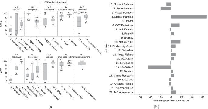
a The score values of EU coastal countries at the indicator level for the most recent year of the assessment period 2012–2022. A box plot and the weighted average values of the exclusive economic zone (EEZ) are shown for each indicator. Country abbreviations¹ are shown for minimum and maximum values, where an asterisk * indicates that more than four countries share the same value. b The EEZ-weighted average change of indicator scores from 2012 to the most recent year (({I}_{EE{Z}_{Avg},MostRecent}-{I}_{EE{Z}_{Avg},2012})). BE Belgica, DE Germany, DK Denmark, EE Estonia, ES Spain, FI Finland, FR France, IE Ireland, LT Lithuania, LV Latvia, NL Netherlands, PL Poland, PT Portugal, SE Sweden, UK United Kingdom.

Full size image

Figure 2b shows the EEZ-weighted average change in indicators from 2012 to the most recent assessment year. Only 13 of the 22 indicators show a positive development. The largest improvement is in Indicator 4. ‘Spatial Planning’, as by now almost all countries have implemented their marine spatial plan, which was also the target of the EU marine spatial planning directive¹⁷. In contrast, Indicator 16. ‘Economies’, which measures the year-on-year growth of established blue economy sectors, presents the largest decline. Since data for this indicator were only available until 2020, this low score could be influenced by the COVID-19-induced decline in economic development. Remarkably, gross value added of coastal tourism decreased by 44% between 2019 and 2020. However, some ecologically important indicators declined as well (e.g. Indicator 2. ‘Eutrophication’ or Indicator 11. ‘Habitat’). Interestingly, fishery-related indicators show a mixed picture. While Indicator 8. ‘Fishing mortality’ (F_MSY/F) improved, Indicator 9. ‘Biomass’ (B/B_MSY) slightly decreased. One reason for this development might be a delayed impact of fishing mortality on biomass levels. Notably, the improvement of the fishing mortality indicator is a more recent phenomenon, as the EEZ-weighted average in this indicator even slightly declined from 2012 to 2016 (by 0.5 points). Thus, it is likely that the overall negative development of biomass is still caused by these previously higher levels of fishing mortality. Furthermore, while adherence to scientific advice has worsened (Indicator 19. SAD/TAC), actual catches comply more with the fishing quota in the most recent year than in 2012 (Indicator 14. TAC/Catch).

Strong versus weak sustainability at the aggregated level

Figure 3a shows the country rankings at the goal level under the two concepts of sustainability for the most recent assessment year. In particular, it compares the ranking under strong sustainability calculated by a Monte Carlo simulation (limited substitution possibilities, σ ~ U(0, 1)) with rankings under weak sustainability, calculated as the arithmetic mean of the target scores (unlimited substitution possibilities, σ → ∞). Countries above the 45° line perform better under weak sustainability, as they can compensate for poor performance in one target with good performance in others. This implies that their level of achievement of SDG 14 is less balanced. For example, France ranks 3rd under weak sustainability but only 11th under strong sustainability. This reflects an imbalance in its achievement of SDG 14, as the country has the second-largest spread between the lowest and highest target scores of all the countries assessed. In contrast, Germany is ranked 5th under weak sustainability, while it is ranked 3rd under strong sustainability. This is the result of a more even distribution of target scores. Compared to other countries, Germany does not have the highest or lowest score for any target and has the third lowest spread between the lowest and highest target score. Under both concepts of sustainable development, Estonia ranks first. The last place is occupied by Finland and Sweden under the concept of weak and strong sustainability, respectively. To see how the rankings change when one of the targets is removed from the calculation, see Supplementary Fig. 3. The information in the figure allows users to derive ranking information in case they consider a target (and the underlying indicators) not suitable for measuring sustainable development. On the other hand, the figure indicates for each country which targets it should focus on to improve sustainable marine development.

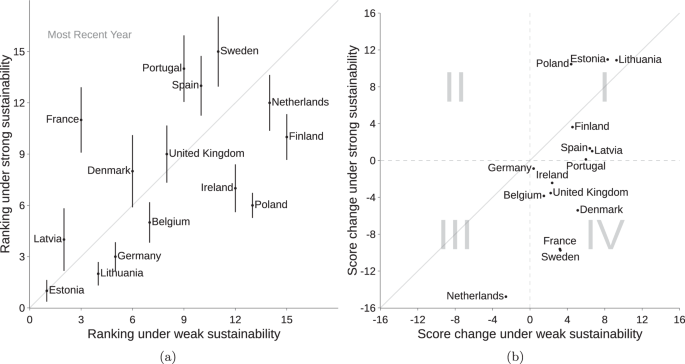
Panel (a) shows the ranking of EU coastal countries under the two concepts of sustainability for the most recent year. Error bars represent the standard deviation under the Monte Carlo simulation calculation of average rank under the concept of strong sustainability. Panel (b) shows the development from 2012 to the most recent year under two concepts of sustainability (CI_{Country,MostRecent} − CI_Country,2012).

Full size image

Figure 3b shows the actual change in scores at the SDG level between 2012 and the most recent assessment year for both sustainability concepts. Quadrant I (III) contains developments where sustainable development is (not) achieved according to both concepts. Quadrant II contains those countries that achieve sustainable development only under strong sustainability, implying a development towards more balanced, but overall lower, target scores. The opposite is true for Quadrant IV. Here, the sum of scores across targets has increased, but their distribution has become less balanced.

Seven countries improve under both sustainability concepts, with Estonia, Lithuania, and Poland leading the way. During the assessment period, Estonia improved on seven of the ten targets. In addition, Estonia worsened its performance on targets that it was already performing well on (e.g., Target 14.4 ‘Sustainable fisheries’) and made large improvements on targets where it was performing poorly. For example, on the acidification target, Estonia improved its ranking on Indicator 6. ‘CO₂ Emissions’ from 15 to 11. Seven countries improved their scores only under the concept of weak sustainability, but not under the concept of strong sustainability, i.e., their aggregated scores increased but their performance became less balanced. France and Sweden are notable, which increased their performance under weak sustainability, but experienced a significant drop when assuming strong sustainability. Overall, the Netherlands is the worst performer, being the only country that fails to achieve sustainable development under both concepts of sustainability.

A comparison of our approach to OHI values (Fig. 4) confirms the robustness of our findings as it allows for comparing across measures subject to different assumptions and interpretations. Both assessments generally provide a similar picture of the marine development of EU countries, although looking at their differences allows for more nuanced insight. OHI generally scores higher or equal to our SDG14 score (except Belgium). In the example of Sweden, Finland, and Spain, these countries exhibit significantly higher scores on the OHI as compared to their scores in our SDG14 indicator. A possible reason could be that these countries have an above-average score in the OHI framework for the goal of protecting ‘Iconic species’. This goal is, however, not assessed under SDG14 as the UN SDG 14 does not distinguish between iconic and non-iconic species. Therefore, we also do not rank species according to their cultural value. The larger variability observed in our results compared to the regionally derived BHI emphasizes the tension field between globally defined SDGs and regional policy needs. Generally, all three approaches largely neglect social equity considerations, and inclusion of this sustainability pillar might alter the results considerably. However, the difference between weak and strong sustainable development, as introduced by our study, clearly shows the extent to which countries perform unevenly across the different goals, demonstrating how our assessment adds information from a methodological perspective to other existing studies.

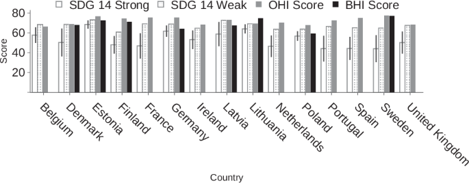
Scores are shown for both concepts of sustainability. The error bars represent the standard deviation under the Monte-Carlo simulation calculation of the average score under the concept of strong sustainability.

Full size image

Putting status and development into perspective

For countries that have already achieved strong performance in the various indicators that measure sustainable development under SDG 14, it becomes more difficult to improve further. Consequently, Fig. 5 puts into perspective the latest status and the progress made between 2012 and the most recent year at the SDG level. Progress is measured by averaging the annual growth rate computed by the slope of a log-linear regression of indicator scores against time for each country. Rather than comparing two points in time, this approach includes all available data points effectively measuring the trend. Status represents the score under the concept of weak sustainability. The dotted lines represent the EEZ-weighted average for both dimensions.

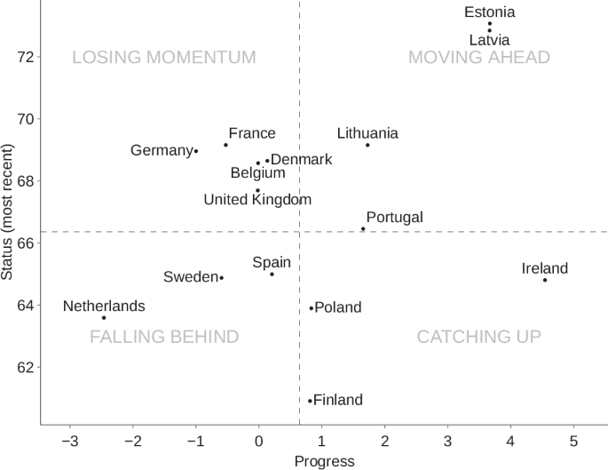
The dashed horizontal and vertical lines are the EEZ-weighted average of the status and progress values, respectively.

Full size image

Countries are grouped into four categories: (i) moving ahead if both status and progress exceed the EU average level, (ii) catching up if the status is still below average but progress is relatively fast, (iii) losing momentum if countries risk their above-average status by presenting low or negative progress, and (iv) falling further behind if both status and progress are below average.

Looking at the top right corner, it is clear that the three Baltic and Nordic countries are progressing. In particular, Estonia has the highest current status and the fastest progress over time. Among other things, its rapid progress is due to strong improvements in Target 14.1 ‘Pollution’, lower eutrophication levels, and higher plastic recycling rates (Indicators 2. and 3., respectively). In addition, its top scores in Target 14.2 ‘Ecosystem-based Management’ and 14.b ‘Artisanal Fisheries’ is a major reason for its high status.

Of the countries catching up, Ireland is the country with the largest average growth rate thanks to a substantial decrease of high-risk subsidies to the fishing industry from 2014 to 2018. The country also relatively increased its coastal population employed in marine-related activities compared to other countries (Indicator 15a). Portugal is another interesting case progressing quickly, with the fifth-highest average growth rate. In particular, it has increased in Indicator 22. ‘IMO Participation Rate’ and has improved in the dimension of fishing mortality (Indicator 8.). However, Portugal is marginally moving ahead since it has the lowest score for Target 14.1 ‘Pollution’ because of high eutrophication levels and high plastic generation per capita. Similarly, low coverage of marine protected areas leads to low scores in Target 14.5 ‘Protection’.

Among the countries losing momentum, Germany is losing the fastest, with the second-largest negative trend just behind The Netherlands. It particularly failed to meet the expected annual growth rate of 1.5% in gross value added (GVA) for several years in the maritime transport and coastal tourism sectors, which together make up 60% of the GVA of the German blue economy¹⁸. Overall, while other countries compensate for negative trends in some indicators with progress in other indicators, Germany presents small values in its positive trends.

Lastly, the Netherlands is falling behind the other EU coastal countries. In addition to a low score on Indicator 20. ‘Artisanal Fishing’, the Netherlands had the greatest losses in Indicator 12. ‘Subsidies’, implying that the percentage of subsidies that risk promoting IUU fishing has increased the most. Further, examples of negative progress can be seen in Target 15 ‘Livelihoods’ due to a sharp drop in GVA per hour worked in the blue economy and increasing eutrophication levels under Target 14.1.

Establishing scientifically reasonable approaches for indicator selection, normalisation (ensuring data comparability), weighting (defining correct interrelationships), and aggregation (obtaining appropriate functional relationships) is essential for developing meaningful Sustainable Development indices^19,20. There may be pronounced differences in the indicators selected when social conditions such as equity and not only resource availability, are considered²¹. Ensuring a more equitable distribution of goods and services provided by the ocean remains a major challenge²², which is often not adequately represented in indicator selection. Instead, growth-based narratives are favoured, while competing discourses are largely neglected²³.

Unfortunately, in practice, selecting indicators suitable to assess a socio-environmental system is constrained by data availability, constituting a normative decision with implications for the outcomes of the composite indicators that represent the sustainability targets. Moreover, we must pay particular attention to scale adjustments and the transformation of highly skewed indicators^19,24,25,26. Consequently, our selection of indicators to measure sustainable marine development is guided by the SDG 14 framework. However, our analysis focuses on blue growth following the concept of Arrow et al.²⁷, focusing on intergenerational equity, but does not delve into the social dimension of sustainable development and intragenerational equity²⁸. While blue growth offers potential benefits such as shared prosperity, food security, local employment, capacity building and economic gains, rapid and uncontrolled development can lead to environmental and social injustices. Overall, ocean-based development activities are likely to result in a mix of positive and negative social impacts for various societal groups²⁹.

The indicators selected do not cover all aspects of sustainable development. By not being able to include relevant indicators because they are not measurable or their data is unavailable, our selection does not always align with the focus of the SDG targets. For instance, by focusing exclusively on the total research budget allocated to marine technology, we fail to consider the broader objective of Target 14.a on marine science to enhance oceanic health and develop sustainable practices (see in this context also the Ocean Decade’s emphasis on enhanced integrated ocean management and the advancement of a sustainable ocean economy³⁰). To cover the comprehensiveness of sustainable development, actions should advance not only biophysical knowledge of the ocean but also its relation to people and their well-being³¹. The SDGs require ocean science to be transdisciplinary, involving collaboration with social sciences, policymakers, and local knowledge holders, effectively reducing power imbalances^31,32.

Our indicator selection also suffers from the ‘country first’ approach which prioritises official country data over secondary sources. Data reported by UN member states, such as the data related to indicators on fish catches (14. and 19.) and fishing subsidies (12.) might not be trustworthy³³. Internationally comparable data remains challenging, and quality and adherence to international standards across countries vary widely. Another constraint is the uncertainty of the effectiveness of certain objectives, such as Target 14.5, which aims to measure “the coverage of protected areas in relation to marine areas”, since the indicators used cannot accurately measure this. In our assessment of this target, the official indicator of Key Biodiversity Areas is complemented by an indicator of Marine Protected Areas (since protected areas have a broader conservation purpose). However, an additional indicator could measure how effective areas are in achieving their protection objectives, which depend on a range of management and enforcement factors³⁴.

A particular issue with the framework designed by the Inter-agency and Expert Group on SDG Indicators (IAEG-SDGs) is that few targets contain more than one indicator. All ten SDG 14 targets are measured using only one indicator each. We try to overcome this limitation by including at least two indicators per target (except 14.c). A limited number of indicators per target can cause wrong incentives and measurements, with indicators prioritising certain aspects of the SDGs over others and failing to capture the full scope of sustainable development³⁵. For example, although Target 14.7 aims to increase economic benefits from the sustainable use of marine resources, its single official indicator measures the value added of sustainable marine capture fisheries as a proportion of GDP. This indicator fails to capture important aspects of sustainable marine resources management such as preserving biodiversity, protecting coastal communities, and ensuring sustainable livelihoods. We try to encompass more aspects of this target by including indicators that measure the livelihoods of the coastal population (Indicators 14a. and 14b.). Yet, our indicators are still limited in measuring intragenerational equity within the economic dimension, a fundamental aspect of sustainable development³⁶.

The normalisation of selected indicators implies some arbitrariness regarding the assessment¹⁹. Despite all indicators being scaled to a range of 0–100 after normalisation, it is striking that some indicators yield high scores for most countries, while others typically result in low scores. This disparity arises due to the varying ambitions across the indicators, defining the targets for normalisation. For example, a country’s performance in indicator 1. ‘Nutrient balance’ is assessed against the top 3 countries with the lowest nutrient balance in Europe between 2012 and 2019. Although outliers have been excluded, this best-practice target still seems highly ambitious, with only one country scoring higher than 50 points. In contrast, official fishing quotas were used as the reference for assessing countries in 15. TAC/Catch, resulting in relatively high scores (no country below 90 points) since this benchmark represents a minimum requirement rather than an ambitious sustainability target.

There is only mixed real-world evidence for the success of the European Common Fisheries Policy (CFP) regarding targets 14.4 ‘Sustainable Fishing’ and 14b ‘Small-scale Fishing’ over the last few years. On the one hand, the European Commission³⁷ states that fishing opportunities improved greatly with fewer stocks being overfished. The European Environment Agency³⁸ recognises that, in general, some stock recovery can be observed. However, not all EU objectives have been met and further action would urgently be needed, something not immediately obvious from our indicator approach. In addition, significant (eco-)regional differences cannot be easily resolved using country-level indicators. A prominent example is the Baltic Sea, with struggling fish stocks and a suffering small-scale fishery³⁹.

When it comes to fisheries, a potential reason for the perceived mismatch of the indicator score and the environmental situation is the system of setting reference points used in the assessment and calculation of indicators, i.e., B_MSY and F_MSY. These indicators are regularly reviewed and adapted in a formal framework, the ICES benchmark process⁴⁰. While this adaptation of the targets is urgently needed to deliver the best available scientific advice, it also blurs the long-term changes in the ecosystem. Ecosystem-driven reductions in stock productivity and, hence, B_MSY are not fully captured in the indicators. Paradoxically, a well-established adaptation system contributes to the blurriness of the indicator and lays the foundation for the shifting baseline syndrome⁴¹.

These considerations show that it is hardly possible to develop a set of indicators considered to be the “true” assessment from the perspective of all stakeholders. On the contrary, the various challenges of measuring, comparing, and aggregating dimensions of ocean health could be addressed by a series of indices that apply different selection, normalisation, and aggregation rules, resulting in a distribution of improvements vs. degradation⁴². The quality and robustness of the assessment improve with time by comparing different assessments and mutual learning. This way, the assessment can support accountability, effective reporting and learning, and evidence-based decision-making and scenario planning⁴³.

Our assessment shows how distinguishing between weak and strong sustainability allows for identifying how far a balanced development is achieved across socioeconomic and ecological dimensions of ocean health. In summary, our analysis supports the view that the EU achieves sustainable marine development, but not comprehensively and across all countries. While seven countries achieved sustainable development under both weak and strong sustainability, seven countries developed only under weak sustainability, and one country did not achieve progress under both concepts. Nevertheless, it is evident that many ocean ecosystem services are provided on a global scale, and are consequently influenced by the collective action of humanity. This is particularly evident in the case of the ocean carbon sink. The objective of our study is to compare EU countries (and how they contribute to the mitigation of global challenges) and not to position these countries in a world ranking. Our focus is on EU policymakers and we are concerned with the pressure countries exert on the system. Regarding the interpretation of the ranking, it should be noted that a high ranking in the EU comparison does not necessarily imply a minor overall contribution to a global problem.

Indicator selection

Several economic and particular natural capital stocks underlying blue growth can only be approximated by indicators⁴⁴. Concerning indicator selection, we prioritised the reliability and availability of data for quantification over longer time horizons and the possibility of deriving political objectives. Accordingly, our indicator selection is guided by the UN Global Indicator Framework. However, the UN SDG indicator base is subject to several limitations. It has been criticised for failing to adequately address the social dimensions of sustainable development and not being as carefully selected and developed as the SDGs themselves^33,35. Furthermore, several proposed indicators (14.1.1, 14.3.1, 14.4.1) in the framework aim at measuring the state of marine resources, preventing the assessment of the pressure put and the progress made by countries. Most indicators (14.2.1, 14.4.1, 14.6.1, 14.a.1, 14.b.1, and 14.c.1) that assess the pressure or response of countries present large spatial and or temporal data gaps or are measured with binary or categorical data, preventing a proper assessment of the progress towards the SDG 14 and comparison between EU countries. Therefore, although we aim to measure the ten official SDG 14 targets, we could not include the official UN indicators besides two exceptions (12. Key Biodiversity Areas, 19. Marine Research). When choosing indicators, we aim to measure the contribution of countries in each target, either using pressure indicators (e.g., carbon emissions per capita instead of average marine acidity) or response indicators (e.g., progress of implementation of Maritime Spatial Planning as an alternative to countries using ecosystem-based approaches to managing marine areas). In some cases, these pressure indicators are complemented with state indicators (e.g., inclusion of eutrophication levels in 14.1 Pollution) for a more comprehensive assessment.

For fisheries-related indicators, we rely on data from the International Council for the Exploration of the Sea (ICES). Target 14.4 ‘Sustainable Fishing’ is measured by both the level of fishing mortality (8. F_MSY/F) and biomass (9. B/B_MSY) in comparison to their level under Maximum Sustainability Yield (MSY) conditions. In addition, we measure adherence to scientific advice when fishing quotas are set by including an indicator that compares scientific advice on catch provided by ICES to the actual Total Allowable Catch (TAC) set politically (19. ‘SAD/TAC’). Finally, indicator 14. ‘TAC/Catch’ measures the adherence of realised catches to the fishing quota. Depending on the year and indicator, 52-75 fish stocks were included in the assessment. Generally, ICES data are obtained at the fish-stock level. To measure the contribution of each country to the state of the fish stock, we calculated catch-weighted averages. For indicators 8., 14. and 19., we take the yearly country catches, but for indicator 9. B/B_MSY we use a seven-year moving average to account for past catches that have led to the depletion of today’s stock. The summary of the indicator selection can be found in Table 1. More information on indicator selection can be found in the supplementary information.

Indicator transformation and aggregation

We apply a difference-to-target normalisation to calculate ratio-scale, fully comparable (RFC) indicators with a [0–100] range (An indicator X_I is ratio-scale measurable if its ordering is unique up to a transformation of this variable by f_i(x) = a_i × x where a_i > 0) which allows meaningful aggregation^19,45. We choose target normalisation because, unlike ratio normalization (e.g. min–max normalization), extremal elements in a data set do not influence normalised values. Since scales work as implicit weights, when the minimum and maximum values are wide apart, they can distort the index scores²⁴. Moreover, target normalisation is free from dramatic changes that occur in ratio normalization when extreme values in the dataset change⁴⁵. Another advantage of target normalisation is its ability to include contextually relevant parameters in the form of baseline and target values. This specificity of a target also helps in interpreting the normalised values. The target values may align with the characteristics and environmental or socioeconomic requirements of the system being studied (e.g., the planetary boundary of maintaining global average CO₂ in the atmosphere at 350 ppm), and they can also be uniform values, such as those outlined in government regulations or organisational guidance (e.g., target 14.5: Conserve at least 10% of coastal and marine areas).

To derive a target for each indicator, we followed a three-step approach: (1) when available, we use a uniform target. This is the case for 11. MPA/EEZ (instead of the UN target, we follow the advice of Schellnhuber et al.⁴⁶: marine protected areas should cover at least 20–30% of the area of marine ecosystems) and for 17. IMO Participation (following Rickels et al.⁴⁷, we choose the maximum number of sea protocols as the target value); (2) In the absence of official targets, we choose targets that align with the environmental system being studied. This applies to fish-related indicators (e.g., fishing mortality in line with MSY for indicator 8.) and for pre-industrial pH level for indicator 7.); (3) As the last resource, we determine a target using the average of the top three performing countries in the dataset. Before calculating this endogenous target, we remove outliers using the interquartile method and choose to consider all EU countries present in the dataset, not only the 15 countries included in this assessment. The reference value derived using this approach can be interpreted as a “best-practice” target. Apart from the benefits of using target normalisation outlined above, setting a benchmark within the EU countries to measure progress aids in developing a policy-relevant assessment.

We apply a generalised mean to incorporate a range of substitution elasticity values that allow us to assess progress under the concept of strong and weak sustainability^48,49. Consider the generalised mean according to social choice theory^19,50 of the form:

where CI_ct is the composite indicator value for country c at time t, I_ict is the value of indicator i for country c at time t, α_it is the weight of indicator i at time t, and σ is the elasticity of substitution between the different indicators, with α_it > 0 and 0 ≤ σ ≤ ∞. Large values of σ translate into high elasticity of substitution, which implies that it is relatively easy to compensate a low score in one indicator with a high score in another indicator (weak sustainability). The opposite is true for small values of σ. As shown in Fig. 6, the composite indicator can be derived from various specific function forms, with the specific form determined by the value of σ.

Depending on the elasticity of substitution, the generalized mean takes on different functional forms, which correspond to different substitution possibilities and concepts of sustainability (adapted from Rickels et al.⁵⁹).

Full size image

By relying on a generalised mean to construct the scores, we ensure the robustness and transparency of the results. By contrasting aggregated scores obtained under the two concepts of sustainability, we can identify unbalanced performance across targets because score values under strong sustainability are more sensitive to left outliers. To understand the implications of this approach, consider two countries whose indicator values sum up to the same amount, but one country has more balanced values. While the arithmetic mean (weak sustainability) returns the same score for both countries, the geometric mean (strong sustainability) returns a higher score for the country with the most balanced values. Instead of assigning weights to specific indicators to differentiate their importance for sustainable development, this method reflects a preference for balanced performance between indicators and targets^47,51.

Considering that the targets are composed of several complementary indicators, we assume that the substitution possibilities between indicators corresponding to a specific target are higher than the substitution possibilities between targets. Following Rickels et al.⁴⁷, we build a nested composite indicator with different substitution possibilities at different steps of the aggregation process. We calculate the target scores under the assumptions σ_target = 10²⁶ and σ_target = 0.5⁵² to compare the results between the two concepts of sustainability. The same procedure is applied to the aggregation at the SDG level, where we assume σ_SDG ≤ 1 for the concept of strong sustainability and σ_SDG → ∞ (perfect substitution possibilities) for the concept of weak sustainability. Instead of choosing a specific value for the case of σ_SDG < 1, we assume σ_SDG ~ U(0, 1) and implement a Monte Carlo simulation (N = 10,000) to obtain a range of scores for the concept of strong sustainability at the goal level.

The composite indicator CI_ct allows us to compare the state of ocean resources and services in the selected EU coastal countries at a specific point in time. By comparing CI_ct in different years (ΔCI = CI_mostrecent − CI₂₀₁₂), we can assess progress over time (see Fig. 2b).

To assess the direction of progress of each country, we calculate the change of trend using the slope coefficient of a log-linear regression for each I_ic against time (ln(I_ict) = a + b_ict) where b is the slope to be estimated and a = I_ic0. To calculate the linear regression, we use all data between 2012 and 2023, with the available data points varying between indicators. The slopes are aggregated at the target and goal level using the arithmetic mean (weak sustainability).

We use the log-linear regression method to estimate the average annual growth rate, similar to Statistics Netherlands⁵³ and the World Bank⁵⁴ because it offers a more comprehensive analysis than the compound annual growth rate (CAGR) used in some SDG assessments, such as those by the United Nations⁵⁵ and Eurostat⁵⁶. While CAGR only considers the first and last data points, potentially missing valuable fluctuations, the linear regression approach uses all available data points, ensuring a more accurate representation of trends. The regression approach is also advantageous for indicators with limited data points, whose trends cannot be measured using the simple average annual growth rate (AAGR) (see Sachs et al.⁵⁷). Despite some limitations, such as assuming linearity and the assumption of uncorrelated residuals in time series⁵³, the method offers valuable insights when combined with score data and supports long-term structural change assessment over temporary variations.