Structural stability changes of the Atlantic Meridional Overturning Circulation

Introduction
Although the increasing trend of atmospheric CO2 proceeds at centennial time scale and in principle it could be reversed, the potential climatic changes it induces could be faster and irreversible, with significant socio-economic impact. Components of the climate system which suffer rapid irreversible transitions between two states could generate this type of response to anthropogenic forcing and are known as tipping elements1.
Paleoclimate reconstructions and simulations indicate that the Atlantic Meridional Overturning Circulation (AMOC), a central climatic tipping component, played a pivotal role in past abrupt changes, during glacial2,3,4 and interglacial periods5. On one side, through its transport of heat and carbon from the surface to the deep ocean it mediates the climatic response to anthropogenic forcing. On the other side, through its redistribution of heat at the surface, the AMOC has a quasi-global heterogeneous climatic impact6,7. Moreover, through its connection with other tipping components, it could induce a cascade of rapid transitions8.
A range of models, from conceptual to General Circulation Models (GCMs), indicate that the AMOC has more than one stable state9,10,11,12,13. Its nonlinear dynamics can be synthesized by the hysteresis diagram reflecting changes between monostable and bistable regimes. The last is characterized by multiple equilibria and irreversible transitions between them, when the forcing overpasses a threshold value9,14,15.
Coupled Model Intercomparison Project Phase 5 (CMIP5) and CMIP6 models show a small decreasing or no significant AMOC trend over the 1850–2005 period and they project a decline between 0% to more than 50% in response to increasing greenhouse gases, by the end of the 21st century16,17,18,19. A collapse of the overturning during this time interval is not projected, in line with stability assessment suggesting that in a majority of models AMOC is currently in a monostable regime20, implying the absence of an abrupt shift between two stable states. Whereas the Fifth Assessment Report (AR5) of the Intergovernmental Panel on Climate Change identifies an AMOC collapse as a low probability event, but potentially with a high impact21, AR6 estimates (with medium confidence) as likely that under stabilization of global warming at 2 °C relative to 1850–1900, it will weaken for several decades by about 20% of its strength and then recover to pre-decline values, over several centuries22.
Direct observational data of AMOC strength, extending over the 2004–2012 period, indicate a slowing down trend which cannot be distinguished from natural variability23,24. Indirectly inferred AMOC variations, for example based on sea surface temperature (SST), indicate that it has weakened over the 20th century25,26, under the influence of increased atmospheric CO2 concentration27, in contrast with numerical simulations28. Long-term reconstructions indicate that AMOC intensity is at the lowest level in the last millennium29. However, the slowdown of AMOC is still a debated topic30,31,32,33.
Observational based estimations of freshwater export suggest that the current AMOC is in a bistable regime34,35 and early warning signals covering the 1905–1985 period applied on AMOC reconstructions indicate that it is heading toward a bifurcation point36, which could be followed by an AMOC collapse during this century37. This is in contrast with the monostable regime indicated by a majority of models and implies large uncertainties regarding our understanding of AMOC past and future evolutions and its present distance from thresholds38,39,40.
Here we address this contrast by searching for common denominators between data and model simulations. Through such an approach we aim to overcome the inherent limitations of the data (quality and length) and model imperfections. We focus on two simulated templates of AMOC dynamics. One of them emphasizes complex changes of the overturning intensity in response to variable freshwater forcing (i.e. Hopf bifurcation, convective and advective hysteresis behavior), but also the SST patterns associated with them15. This facilitates comparisons with observed SST modes linked with AMOC changes. A second simulated template used here is provided by integrations of conceptual box models, which were shown to catch the AMOC dynamics simulated with a general circulation model41. They emphasize two types of tipping, Bifurcation-induced (B-tipping) and Rate-induced (R-tipping), but also provide criteria used to diagnose if AMOC overpassed a critical point, based on bifurcation diagram and phase space representations. In principle, these could be also reconstructed based on observational data. Having the goal to infer potential structural changes of AMOC dynamics based on instrumental data, our strategy is to search for correspondences between simulated templates and observed modes linked with overturning dynamics.
Results
Analogy between simulated and reconstructed AMOC dynamics
Decadal and longer AMOC fluctuations can be reconstructed through a linear combination of two modes with distinct projections on the Atlantic SST field27. These modes were emphasized also in numerical simulations17,42 and are identified here through Empirical Orthogonal Functions (EOF) analysis of the observed North Atlantic (80°W-20°E, 0-80°N) annual SST anomalies field, from the HADISST1 dataset43 (see Methods) (Fig. 1). They are distributed over a 1° × 1° grid and extend over the 1870–2023 period. In order to remove the direct effect of global warming on the Atlantic SSTs, the spatial global average of each year is subtracted from the values in all points of the corresponding grid.

a Spatial pattern of the Trend Mode (degree C), explaining 32% of variance; b Spatial pattern of AMO (degree C), explaining 17% of variance; c Normalized time-component of the Trend Mode (indigo line) and its 23-yr period oscillatory signal, isolated with SSA (red line); d Normalized time-component of AMO (indigo line) and its 23-yr period oscillatory signal, isolated with SSA (red line), The modes were derived through EOF analysis of the North Atlantic SST field of annual means of anomalies, extending over the 1870–2023 period (see Methods).
As indicated by a previous study44, whereas one is associated with a centennial-scale decreasing AMOC trend (hereafter SST-AMOC-Trend Mode) and with deep water formation (DWF) in the Nordic Seas, the other is associated with multidecadal variations (Atlantic Multidecadal Oscillation – AMO) (hereafter SST-AMOC-AMO), linked with DWF in the Labrador and Irminger Seas, with the latter appearing to play a more prominent role for the overturning than the former45. One notes that SST-AMOC-TM was derived also based on an EOF analysis of SST reanalysis field extending over the 1600–2000 period46 (see Methods). Its time component includes a pronounced decreasing trend starting at the end of the 19th century, aligned with the corresponding time series derived based on observations (Supplementary Fig. 4). Therefore, the decreasing trend appears to be a unique feature of SST-AMOC-TM since 1600. In order to investigate the relevance of the two SST-AMOC modes for the simulated AMOC dynamics, we investigate the spectral content of their time components and compare their spatial SST structures with that corresponding to transitions between different states of the Atlantic overturning, emphasized in model integrations15.
Spectral analyses of the time-components of the two observed SST-AMOC modes include an oscillatory signal with a 23-year period (Supplementary Fig. 2). This bidecadal component was separated through Singular Spectrum Analysis (SSA) of the time components of the two SST-AMOC modes (Supplementary Figs. 2, 3, Fig. 1c, d). SSA is an effective method to isolate nonlinear trends and quasi-periodic components with varying amplitudes in time series47. The last five maxima of the bidecadal signal are synchronized with local maxima of the SST-AMOC-AMO time component (Fig. 1d).
One notes that the AMOC response time (about 8–10 years) to North Atlantic density anomalies48,49,50 is approximatively equal with half the period of this oscillation and that the surface temperatures are in phase with the overturning at decadal and longer time scales51. Consequently, this oscillation is interpreted here as resulting from the AMOC-temperature negative feedback (Supplementary Note 4), consistent with previous numerical studies in which an oscillation with a very close periodicity (22-year period) was emphasized as a self-sustained oscillation49,50. An oscillatory signal with the same period emerged from a Hopf bifurcation in numerical simulations with an ocean model15.
In order to further compare properties of simulated and observed AMOC variability, the bidecadal and multidecadal signals are separated through SSA of the time-components of the instrumental multidecadal mode (Fig. 2a, c; Supplementary Fig. 2j, f) and SST composite maps are constructed based on these isolated time components (Fig. 2b, d) (see Methods). The spatial structures of these two composite maps are compared with corresponding patterns derived from numerical simulations15. Both, the simulated15 (Fig. 6 in that study) and the observed (Fig. 2b) SST maps of the bidecadal mode are marked by a center of maximum anomalies located around Newfoundland. These are expanding eastward in the SST structure associated with the Labrador/Irminger convection changes in simulations15 and with AMO in observations (Fig. 2d), which was also linked with convection in this area44 (Dima et al.).
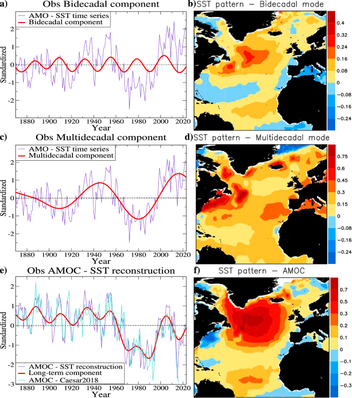
a AMO time series (thin indigo line) and its bidecadal component (thick red line); the last one explains 9% of variance; b SST composite map of the bidecadal oscillation shown in panel (a); c AMO time series (thin indigo line) (as in Fig. 1d) and its multidecadal component (thick red line); the last one explains 52% of variance; d SST composite map of the multidecadal component shown in panel (b) (thick red line); e Sum of time-components associated with SST-AMOC-TM and SST-AMOC-AMO (Fig. 1c, d); the reconstruction based on the trend, multidecadal and bidecadal components is shown in thick red line; an AMOC reconstruction26 is also shown with turquoise line. (see Methods); f Sum of SST patterns associated with TM and AMO (Fig. 1a, b).
Furthermore, as AMOC variations are forced by DWF in both North Atlantic main sites, Nordic Seas and Labrador/Irminger Seas, the SST pattern and time-component associated with AMOC variations at decadal and longer time scales is reconstructed through the superpositions of the spatial structures and time-components of the two SST-AMOC modes, which were linked with these two convection areas44 (Fig. 2e, f). In simulations15 the SST pattern corresponding to the transition between the strong and weak AMOC states is marked by maximum anomalies located at the latitude of the subpolar gyre, with decreasing values southwestward and northeastward from them15. A similar SST spatial structure is associated with the observed integral AMOC mode (Fig. 2f).
In order to infer the relevance of the observed AMOC reconstruction for the Atlantic stream-function variability (Fig. 2f), we use a simulation with an ocean model for the 1958–2009 period52,53 (Supplementary Note 3). Based on the simulated fields we associate the SST-AMOC-TM mode with a bipolar stream-function pattern extending from 60°N to 30°S (Supplementary Fig. 6) and the SST-AMOC-AMO with a stream-function cell centered at 30oN (Supplementary Fig. 7). The simulated integral mode resulting from the superposition of these two modes explains 70% of the annual zonal mean Atlantic stream-function variability in the model integration and its time component aligns well (Supplementary Fig. 8) with the observed SST-based AMOC time series (Fig. 2e), reconstructed based on the SST-AMOC-TM and SST-AMOC-AMO (Fig. 1). Therefore, according with this model simulation, the observed SST-based AMOC reconstruction represents a good approximation of the AMOC variability. One notes that our AMOC index is also significantly correlated (0.80) with another observed SST-based AMOC reconstruction, which was derived through a distinct method and which was linked with the Atlantic overturning changes, as simulated with a CMIP5 ensemble26.
These one-to-one correspondences and close resemblances between the simulated and observed SST-AMOC bidecadal, multidecadal and integral (SST-AMOC-TM+SST-AMOC-AMO) modes (Fig. 2b, d, f) lead, through analogy with model integrations15, to several inferences about AMOC dynamics over the observational period:
-
1.
the very close similarities between the characteristics (periodicity and structure of SST pattern, with the last including maximum anomalies close to Newfoundland, which extend eastward) of the simulated 23-year period oscillation emerging from a Hopf bifurcation of the AMOC’s strong state and that of the observational bidecadal mode (Fig. 2a, b), which manifest over the 1854–2023 time interval (Supplementary Fig. 3), indicates that the latter resulted from a similar bifurcation, which manifested before 1854;
-
2.
the fact that in the simulated hysteresis diagram this bidecadal limit cycle manifests in the right edge of the bistable sector, in the proximity of the tipping point, at maximum distance from the monostable regime of the strong state, implies that at least since 1854, AMOC states reflected by observational SSTs have been also located in this regime, an inference which is supported by previous studies34,35;
-
3.
the resemblance between the SST pattern associated with Labrador/Irminger convection changes in numerical integrations and the structure of the observed SST-AMOC-AMO pattern (with maximum anomalies located around New Foundland, with positive loadings expanding in all directions across North Atlantic eastward) (Fig. 2d), indicates that the latter is associated with convective hysteresis of AMOC linked with DWF in the Labrador/Irminger Sea, an inference which is supported by previous investigations suggesting that SST-AMOC-AMO is linked with DWF in this convection area44;
-
4.
in numerical simulations the SST pattern of the AMOC transition between its strong and weak states15 (Fig. 6 in that study) is similar with that of the observed combined SST-AMOC-AMO and SST-AMOC-TM integral mode (with maximum anomalies located southeast from Greenland and expanding northeastward and southwestward) (Fig. 2f); this resemblance, together with the fact that the former SST-AMOC mode is linked with convective hysteresis, implies that the latter is associated with advective processes, which is consistent with the characteristic centennial scale of the associated time component (Fig. 1c).
The fact that two ((2) and (3)) of the previous four inferences are supported by previous studies, suggests that the analogy between the simulated templates and the observed SST-AMOC modes provides valid information about the dynamical properties of the later modes. The relevance of these inferences indicates that further analogies could be explored and therefore these are extended here to convective and advective hysteresis diagrams.
Convective and advective hysteresis representations
In model integrations the hysteresis diagram is constructed by tracking the AMOC equilibrium response to slow changes in North Atlantic freshwater forcing15. One source of buoyancy is linked with the Arctic sea ice extent, which shows a strong decline during the last decades54 and which was shown to affect AMOC in model integrations through both, freshwater and heat fluxes55. We aim to derive a potential buoyancy forcing index for the overturning based on the dominant modes of Arctic sea ice concentration (SIC) variability56. A forcing time series, with an increased signal-to-noise ratio, is obtained through the superposition of the time-components associated with the first three SIC modes, which are identified through an EOF analysis of the average June-July-August-September fields, extending over the 1870–2017 period (see Methods). These first three EOFs are explaining together 52% of variance and their time components are marked by centennial and multidecadal variations (Supplementary Fig. 9), which are also characteristic for the two SST-AMOC modes (Fig.1c, d). This time series (Fig. 3a) (hereafter SIC-Forcing index) is considered forcing for the SST-AMOC-AMO, which was linked with the Labrador/Irminger Sea DWF57. It shows high positive anomalies between the 1950s and 1970s, with a pronounced maximum around 1968, which could be linked with the Great Salinity Anomaly (GSA), an influx of freshwater from the Arctic in North Atlantic, which propagated over this sector during the 1960s and 1970s58. Using the Information Flow method59 we infer that the SIC-Forcing index has causal influences on the time components of the SST-AMOC-AMO and SST-AMOC-TM modes (see Methods). These results are supported by numerical simulations indicating that Arctic sea ice can affect AMOC at decadal and centennial time scales, through freshwater and heat fluxes55.
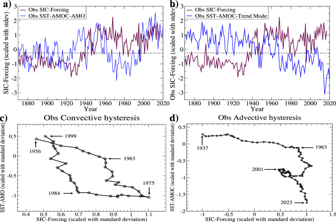
a SIC related buoyancy forcing index obtained as a linear combination of the time-components associated with the first three Arctic SIC modes (dark red line) and the reconstructed SST-AMOC-AMO index (blue line); b SIC related buoyancy forcing (dark red line) and the reconstructed SST-AMOC-Trend index (blue line); all timeseries in panels (a, b) are scaled with their standard deviations; c Convective hysteresis diagram constructed as a bidimensional representation of SST-AMOC-AMO time-component as a function of the SIC-Forcing index; d Advective hysteresis diagram constructed as a bidimensional representation of SST-AMOC-TM time-component as a function of SIC-Forcing index; before constructing the representations in panels (c, d), a 25-years running mean filter was applied to all time series; the representation is constructed with SST-AMOC timeseries lagging the SIC-Forcing index with 10 years; the years marked in the figure reflect the temporal evolution of the SST time series (see Methods).
A two-dimensional representation is constructed, with the time series of the SST-AMOC-AMO mode (Fig. 1d), for the 1956–1999 period, as a function of the SIC-Forcing index (Fig. 3a). This time interval is chosen because it covers the most recent complete AMO cycle (Fig. 1d) and therefore also a closed hysteresis curve (Fig. 3c). In order to consider the delayed AMOC response to freshwater fluxes, a lag of 10 years between the latter and the former time series is used to construct the representation, as indicated by previous studies48.
The sensitivity of the shape of the diagram to the lag used, was investigated by constructing representations using delays between 6 and 16 years (Supplementary Fig. 10). The general shape of the diagram and its main characteristics are preserved for lags in this interval, implying that the main properties of the reconstructed convective hysteresis are robust relative to reasonable variations of the lag used, in a range consistent with previous studies49,60,61. We investigated also the sensitivity of the shape of the diagram to the applied filter length (Supplementary Fig. 10). The key characteristics of the bifurcation diagram, are visible for the reconstructions with running mean filters of 11-year, 15-year, 21-year, 25-years and 31-year length. Therefore, although the smoothing is necessarily in order to remove high frequency variations, the main properties of the diagram are preserved for reasonable variations of the filter’s length. Furthermore, we estimated, by randomly shifting the time series, that the probability to construct a similar diagram with that derived from simulations15 is less than 0.01 (Supplementary Note 5).
The diagram, which is assimilated with a convective hysteresis curve, includes a decreasing strong AMOC state which ends in 1963, followed by a two-step (sharp and mild) decrease toward a weak state, which extends between 1975 and 1984 (Fig. 3c). The loop is closed with a rapid increase toward the strong AMOC equilibrium. All these observed specific properties of the shape of the curve correspond accurately to that of the simulated AMOC convective hysteresis loop associated with DWF in the Labrador Sea15.
This is consistent with the causal influence of the SIC-Forcing on AMOC indicated above by the Information Flow method and validates the inferences based on the similarities between the observed and simulated overturning dynamics. As the convective hysteresis is located in the bistable regime in simulations15, the reconstructed diagram also supports the previous inference that AMOC has been in the bistable regime since at least 1854. Also, it opens the possibility to reconstruct a branch of the advective hysteresis based on the SIC-Forcing index and the SST-AMOC-TM time-component. One notes that the transition from the strong to the weak state of AMOC is essentially linked with advective processes9.
In a similar manner (using also a 10-yr lag), a second diagram is constructed by representing the time-component of the SST-AMOC-TM (for the 1937–2023 period), which was associated above with advective processes, as a function of the SIC-Forcing index (Fig. 3b). The resulting curve includes a mild decreasing trend from 1937 to 1963 (Fig. 3d). After a turning point corresponding to this last year, the curve shows a higher decreasing rate to 2023, with a fluctuation between 1980 and 2013, which is related to the bidecadal cycle which manifest between 1990 and mid-2010s in the SST-AMOC-TM time series (Fig. 3b). However, it does not interrupt the long-term decreasing trend, which continues to manifest after it. Such interdecadal fluctuations in North Atlantic can mask longer-term AMOC changes62. The start of the relatively fast descending branch, located around 1963 in the diagram, could be related to the GSA58.
Early warning signals
In order to investigate a potential tipping around 1970, Early Warning Signals (EWS) (lag-1 autocorrelation, variance, return rate and power of dominant frequency) were computed for two SST-based AMOC reconstructions, the longest of them extending over 170 years (Fig. 4) (see Methods). One notes that it was suggested that EWS computed based on direct AMOC measurements or on indirect measures based on SST are equally relevant63.
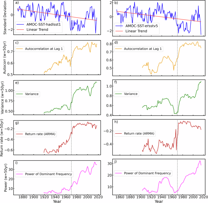
AMOC reconstruction (blue line) based on HadISST1 (a) and ERSSTv5 (b) datasets, with fitted linear trends (red lines); Lag-1 autocorrelation (c, d), Variance (e, f), Return Rate (g, h) calculated as an ARMA process and the Power of the dominant frequency (i, j) for the two AMOC reconstructions. All Early Warning Signals are calculated with a sliding window of length w = 50 years, plotted at the end of the window. The dashed vertical line marks the year 1970. All indicators have a linear fit before and after 1970 with its slope and p-value indicated in the legend. The solid vertical lines in panels (c–f) are marking local maxima of EWS.
A bifurcation-induced tipping (B-tipping) of AMOC implies a gradual increase of the freshwater forcing, followed by a crossing of the saddle-node, which is preceded by critical slowing down of the underlying system. This phenomenon is a consequence of a decrease of the stability of the equilibrium state, signalized by increasing EWS values before the bifurcation point64. From this perspective, assuming that a potential bifurcation will be reach in the future, increasing amplitudes of several EWS toward 1980 were reported36, which are reproduced also in our analyses (Fig. 4), have been interpreted as an indication that the Atlantic overturning state is approaching a B-tipping point. The analysis was questioned65 and answered66.
Alternatively, due to a large rate of change in the forcing, AMOC could not track its strong equilibrium state and it may suddenly move to a different state, through a rate-induced tipping67. Based on box models simulations41 and on general circulation models68,69,70, it was suggested that this type of AMOC tipping is possible. Unlike B-tipping, this type of critical transition is not preceded by a loss of stability, which implies that early-warning indicators do not show significant increases in amplitudes before R-tipping71. However, based on the saddle-node normal form with additive noise and a ramped shift of the equilibrium, it was shown that increases in autocorrelation and variance for this type of critical transition are delayed relative to the shift, with the lagged maximum of the former preceding that of the later variable71. Our analyses show a pronounced increase of autocorrelation and variance, with the former emerging just before 1970 and the latter after this year (Fig. 4c–f). Also, maxima of these EWS are observed after 1970, with that of autocorrelation preceding that of variance. All these features, which are also reproduced by other two EWS, return rate and power of dominant frequency (Fig. 4g–j), were associated with R-tipping71. Therefore, the EWS on SST-based AMOC reconstructions are consistent with an R-tipping of the overturning, manifested around 1970, likely in response to the GSA.
Simulated and observed stream-function and sea surface salinity modes
We further investigate this potential R-tipping of AMOC by searching for similarities with template bifurcation diagram and phase-space representations, provided by numerical simulations, in which salinity plays a major role41. Therefore, we identify the dominant modes of simulated Atlantic meridional stream-function changes and observed sea surface salinity (SSS) variability and relate them to the previously identified SST-AMOC modes.
Stream-function fields derived from a simulation with an ocean circulation model were analyzed in order to identify the dominant modes of variability. The Finite-Element Sea-Ice Ocean Model (FESOM) is integrated in a regionally focused, but with a globally coverage model setup. It has a spatial resolution of up to 7 km, and the simulation extends over the 1958–2009 period52,53. The model set-up is designed to study the variability in the deep-water mass formation areas and was therefore regionally better resolved in the convection areas, in the Labrador Sea, Greenland Sea, Weddell Sea and Ross Sea. In control integrations with FESOM the DWF in the Labrador Sea compares well with observations and therefore the model is suitable in investigations of the large-scale impact of convection in this area.
The EOF analysis of the Atlantic (30°S-80°N) annual means zonally averaged stream-function reveals two dominant modes associated with AMOC changes (see Methods). Whereas one includes two-cells and is associated with centennial variations (Fig. 5b, c), the other is marked by one dominant cell and it is linked with multidecadal fluctuations (Supplementary Fig. 14b, c). Very similar modes were shown in simulations with the IPSL-CM5A-MR climate model72. Therefore, they represent common types of manifestation across monostable (FESOM) and bistable (IPSL-CM5A-MR) AMOC regimes20.
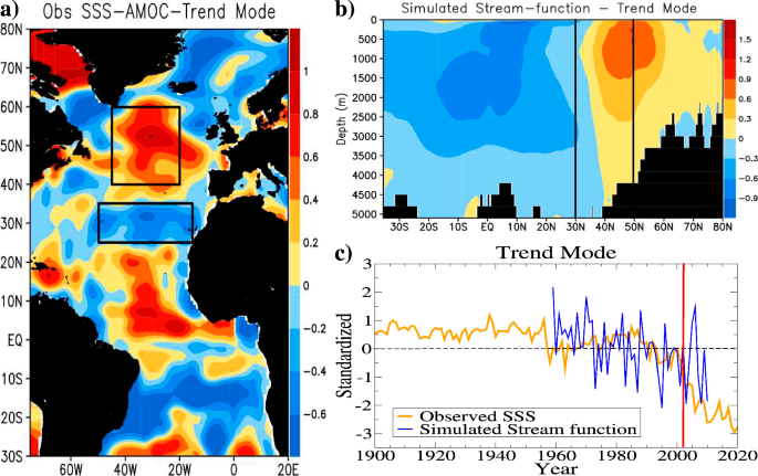
a Dominant SSS mode (units less), explaining 21% of variance; b Dominant stream-function mode (Sv), explaining 60% of variance; c Standardized time-components of the dominant SSS (orange line) and stream function modes (blue line) (see Methods). The rectangles in panel (a) are marking the areas for which are computed SSS indices; the centers of these rectangles are marked by lines in panel (b).
In order to investigate potential links with surface salinity changes, two dominant modes are separated through an EOF analysis of the Atlantic basin (75°W-20°E, 30°S-80°N) SSS anomalies, extending over the 1900–2020 period (see Methods). The pattern of a centennial scale mode (hereafter SSS-AMOC-TM) is characterized by a succession of consecutive centers of SSS anomalies with alternating signs, from the tropics to high latitudes (Fig. 5a). The corresponding time-component is marked by a decreasing trend manifested since the 1980s, which is aligned with the time series of the simulated stream-function AMOC trend mode (Fig. 5c). The maximum correlation between them is 0.48, when SSS lags the later by 14–20 years, with the delay growing as high frequencies are filtered out (Supplementary Fig. 16). The negative SSS anomalies in the subpolar North Atlantic and the positive values in South Atlantic of this mode were linked with accelerated AMOC weakening since 1980s62,73.
The associated stream-function pattern includes a cell centered in the subpolar North Atlantic and another one centered in the subtropical South Atlantic (Fig. 5b). The weakening subpolar one, presumably with contribution from the increased freshwater forcing linked with SIC changes, implies reduced northward salinity advection from lower latitudes, which therefore decreases in the subpolar gyre and accumulates in the subtropics, consistent with the North Atlantic structure of this SSS mode (Fig. 5a). The resulting increased water density in the subtropics implies anomalous downward motion in this region, as part of both North Atlantic subpolar and South Atlantic anomalous cells, which are thus intensified, in opposite directions. The North Atlantic stream-function structure (Fig. 5b) and the SSS hemispheric latitudinal contrast (Fig. 5a) are typical components of the salinity-driven regime of AMOC9. The increased south Atlantic cell leaves negative salt anomalies in the northern tropics. Therefore, both cells are involved in the positive salinity-advection feedback of the North Atlantic, linked with anomalous downward motion in the subtropics, which amplifies an incipient weakening of the polar cell.
This mode is the AMOC-TM footprint on SSS and it is affected by increasing atmospheric CO2 concentration field (hereafter SSS-AMOC-TM)27,74. Therefore, it can be considered an anthropogenic mode. The bipolar stream function structure of the AMOC-TM (Fig. 5b) is similar with that corresponding to the weak state of AMOC, simulated with an eddy-permitting climate model75. One notes that the time-component of the tropical part of the SSS-AMOC-TM (Supplementary Fig. 18) shows a steep decline in the early 2000s, when the meridional SSS gradient starts also to significantly increase (Supplementary Fig. 17).
Reconstructed bifurcation diagrams and phase-spaces
A characteristic picture of simulated AMOC dynamics is provided by bifurcation diagrams, showing the distribution of its states as a function of buoyancy forcing41. Given that the overturning weakening trend is linked with advective processes, with the subpolar AMOC cell, with the SSS-AMOC-TM mode and with the subtropical-subpolar salinity gradient, SSS indices are computed as average values over the regions 50°W-15°W, 25°N-35°N (hereafter Ssubtrop index) and 45°W-20°W, 40°N-60°N (hereafter Ssubpol index) (Fig. 6a, b). In order to increase the signal-to-noise ratio, the long-term components of the two salinity indices and of the SIC-Forcing time series were isolated through Singular Spectrum Analysis, which is an effective method for separating nonlinear trends and oscillatory signals47 (Fig. 6a, b). Based on them are constructed two bidimensional representations, for Ssubpol and Ssubtrop indexes, respectively, as functions of SIC-Forcing time series, which are assimilated with bifurcation diagrams. As for the case of hysteresis diagrams, we consider that AMOC responds to North Atlantic surface density changes in about 10 years48. A cross-correlation between the time series of AMOC-TM and of SSS-AMOC-TM (Fig. 5c), indicates that the latter lags the former with a lag in the 12–22 years interval, depending on the applied temporal filter (Supplementary Fig. 16), from which we use a value of 14 years. Consequently, we use a delay of 24 years between the SIC-Forcing and the two SSS indices to construct the two diagrams.
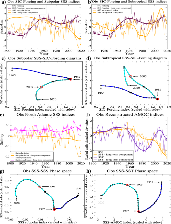
a The SIC-Forcing, the subpolar SSS indexes and their long-term components, identified with SSA; b The SIC-Forcing indexes, the subtropical SSS indexes and their long-term components, identified with SSA; c Bidimensional representation constructed based on the long-term components shown in panel (a), scaled with their standard deviations; d Bidimensional representation of the reconstructed long-term components shown in panel (b), scaled with their standard deviations; in panels (c, d); the representation is constructed using a 24-year lag between SIC-Forcing and SSS subtropical index; the years marked in panels (c and d) correspond to the SSS time series; e Salinity indices constructed as averages over the 45°W-20°W,40°N-60°N (subpolar index-orange line) and over (50°W-15°W,25°N-35°N – subtropical index-magenta line) areas computed based on annual SSS fields; their long-term components were separated with SSA; f SST- (violet line) and SSS-(orange line) based reconstructed AMOC indexes; the long-term component of each index was isolated with SSA; g Bidimensional representation of subtropical index vs. subpolar index, previously normalized with their standard deviations; h Phase space reconstruction based on the long-term components of SST- and SSS-based AMOC indexes, which were scaled with their standard deviations (see Methods); in panels (c, d, g, h) whereas the first thick red circle is associated with R-tipping, the second is linked with the activation of the AMOC-salinity feedback.
The shapes of the (Ssubpol, SIC-Forcing) bifurcation diagram (Fig. 6c) is similar with a part of the corresponding representation shown in numerical simulations41 (Fig. 6 in their study), which resembles a part of the hysteresis shape of AMOC dynamics in response to freshwater forcing9. This representation is marked by an inflection point corresponding to the SSS value in 1987, which separates two descending branches of salinity. In the context of the stream function and SSS modes, it was inferred that the long-term salinity anomalies follow AMOC with a lag of 12–22-years (Supplementary Fig. 16). This implies that the year of inflection derived from SSS-SIC-Forcing representations, 1987, reflects AMOC changes around 1970. Around this last year the overturning shows a sharp decrease (Fig. 2e). SSS weakens with increasing SIC-Forcing index before the inflection point, but also afterward, although the freshwater forcing decreases. The fact that SSS gets further away from the strong state although the freshwater forcing decreases, indicates that at the inflection point AMOC escaped the attractor of its strong state, likely in response to GSA, through an R-tipping, as indicated by EWS (Fig. 4). The shape of the (Ssubtrop, SIC-Forcing) bifurcation diagram (Fig. 6c) includes also an inflection point associated with year 1987 and resembles also closely the corresponding representation shown in numerical simulations41 (Fig. 6 in their study). The representations suggest that after the tipping point, whereas that salinity decreases in the subpolar North Atlantic, it accumulates in the subtropics.
Another bidimensional representation (Ssubtrop, Ssubpol) is constructed based on the long-term components identified with SSA in the two records (Fig. 6e). The diagram shows a change in the curvature from clockwise to anticlockwise, around 1987 (Fig. 6g). Such a change indicates an approach to the lower branch of AMOC and that a tipping point have been already passed41.
This bidimensional space reconstructed based on two SSS time series is topologically equivalent with the full attractor associated with the AMOC dynamics76. The fact that SST influences also the water density, which is a driver of AMOC changes, implies that temperature is also a key variable of the attractor. Through the Takens’ theorem76, this opens the possibility to reconstruct another bidimensional phase space, based on SSS and SST time series, which are interdependent variables linked with AMOC changes. This second representation is also topologically equivalent with the full attractor of AMOC dynamics. Therefore, in order to test the robustness of the shape of the phase space representation constructed using two SSS time series, we aim to reconstruct a second one based on surface salinity and temperature.
It was shown that AMOC changes at decadal and longer time scales results from the superposition of the two modes (SST-AMOC-TM and SST-AMOC-AMO)27. Here these were identified in both, the Atlantic SST and SSS fields (Figs. 1, 5 and Supplementary Fig. 14). Through the superposition of the time-components of these two modes, derived separately from the SST and SSS fields, are reconstructed two AMOC indices, for the 1900–2020 period, corresponding to these two variables (Fig. 6b). The SST index shows interdecadal fluctuations, in contrast to the salinity time series, which reflects longer-term changes only. The second phase-space, reconstructed based on these two, SST and SSS based AMOC indices (Fig. 6h), shows a very similar change in curvature around 1987, as that emphasized in the phase-space constructed based on the two salinity indices (Fig. 6g). This close similarity indicates that the change in curvature is a feature of the phase space representation of the AMOC dynamics and that it is not sensitive to the data or method used to reconstruct it.
Discussion
Analogies between simulated overturning dynamics15 and observed SST-AMOC modes (Fig. 2) indicate that whereas SST-AMOC-AMO is related to convective processes, SST-AMOC-TM is associated with advective phenomena. The processes of this last type are responsible for the transitions between the strong and weak states of AMOC9. The analogies also indicate that the overturning suffered a Hopf bifurcation before 1854 and that at the latest since that time it has been in the bistable regime. Based on observational SST data, together, the reconstruction of a branch of the advective hysteresis diagram (Fig. 3d), the very limited increases in EWS before 1970 and their maxima after this year (Fig. 4), the shift of the SSS-AMOC-TM mode (Supplementary Fig. 18d), the reconstructed bifurcation diagrams and phase-spaces (Fig. 6), suggest that the overturning suffered an R-tipping around 1970 (Fig. 7).
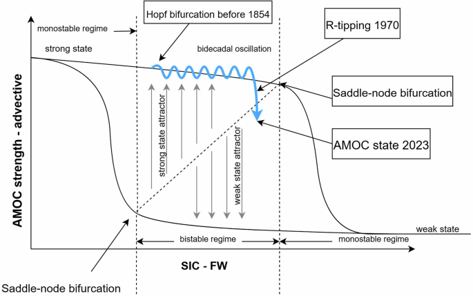
These changes are Hopf bifurcation before 1854, the manifestation of the bistable regime, an R-tipping around 1970 and the belonging of the 2023 AMOC state to the weak state’s attractor.
The SST-based reconstruction of AMOC indicates that it suffered a sharp decrease around 1970, likely in response to GSA77 (Fig. 2e). As freshwater anomalies related to GSA continue to propagate over North Atlantic through the 1970s and early 1980s58, the bidecadal cycle is almost suppressed until early 1990s, when AMOC reaches the lowest level since 1870 (Fig. 2e). The weak overturning at that time implies reduced northward heat transport and negative (positive) temperature (density) anomalies in North Atlantic, which are followed a decade later, in the 2000s, by a high positive amplitude of the bidecadal cycle (Fig. 2e). Therefore, this large amplitude could be considered a consequence of the sharp reduction of the overturning around 1970, through the effect of the AMOC-temperature negative feedback. One notes that the long-term decreasing trend of the advective time component of the overturning continues to evolve during this period and reaches a record minimum during the 2010s (Fig. 1c).
In case of a B-tipping, the buoyancy forcing would increase slowly until AMOC crosses the saddle node into the attractor of the weak state. At that point the salinity-advection feedback is already intense enough so that the salinity mode is stronger than the temperature one9. Unlike this, although the saddle node was not yet reached, around 1970 AMOC decreased sharply in response to a rapidly increasing freshwater forcing related to GSA. Through R-tipping (Fig. 2e), it escaped the strong state attractor and entered the weak state’s basin (Fig. 6c, d, g, h). Whereas the SST response to AMOC changes is relatively fast (1–3 years), the adjustment time of SSS (and of the salinity-advection feedback) to reduced overturning is relatively slow (about two decades) (Supplementary Fig. 16) and salinity has a back-impact on ocean circulation in about one decade48. Consequently, about three decades after the 1970 R-tipping, in the mid-2000s, the intensity of the salinity-advection feedback is adjusted to the reduced AMOC strength and starts to increase significantly (Supplementary Fig. 17). At this time the SSS-AMOC-TM starts also to decrease at a high rate (Fig. 5c and Supplementary Fig. 18b, d), while the overturning is attracted to its weak state. Consistent with these, it was reported a salinity pileup in South Atlantic as an indicator of an accelerating AMOC weakening in the last decades73, which is masked in the North Atlantic “warming hole” region by “noise”, represented by interdecadal variability62. Therefore, the climatic impact of the AMOC transition toward the weak state, which starts to accelerate during the 2000s, is yet partially masked in North Atlantic by decadal fluctuations, likely related to the AMOC-temperature negative feedback49,50,78. The tipping and the accelerated weakening of the advective component of AMOC after activation of the salinity-advection feedback is supported by reports of observed significant cooling of the upper ocean North Atlantic after 200579, of decreasing salinity trends in the subpolar North Atlantic after mid-200080 and by direct AMOC measurements indicating its weakening since 2004, in association with the SST-AMOC-TM pattern81.
Superimposed on the centennial weakening trend of the overturning (Fig. 1c), likely induced by the largest atmospheric CO2 concentration over the last 800,000 years27,82, the late 1960s GSA represents a rapidly increasing freshwater forcing, unprecedented in the 20th century. Both forcing factors could contributed to an R-tipping of AMOC and to its millennial record low strength reached in the last decades29. In this potential scenario, an AMOC collapse by the impact of the salinity-advection feedback and further buoyancy forcing from the Arctic sea ice and Greenland ice-sheet, in a time horizon of decades83, cannot be excluded.
As AMOC is a central tipping component, connected with other critical climatic systems which could be destabilized to overpass thresholds, its irreversible transitions could generate a tipping cascade, with quasi-global impact8. These results underline the need for a long-term temporal assessment of the AMOC stability on multi-centennial to millennial time-scales, since the possibility that it already approached the attractor of its weak state cannot be excluded.
Methods
Isolating climate modes using the EOF method
A climate mode can be defined as a set of coherent processes associated with distinct spatial and/or temporal patterns. The Empirical Orthogonal Functions (EOF) method decomposes the multidimensional input field in a series of mathematically orthogonal spatial patterns (EOFs), which constitute a new base in which the initial data can be represented. By projecting the EOFS on the initial field one obtains their associated time components (or principal components – PCs).
The (mathematical) orthogonality between patterns could be considered an indication that distinct EOFs are associated with corresponding processes, which are physically independent from each other. This could be interpreted as an indication that the respective EOFs are linked with different climate modes. If this inference would be generally valid, it would imply that distinct EOFs correspond to different climate modes. However, two EOFs with distinct structures could be associated with the same climate mode, as it is suggested by a particular example.
Let consider an oscillatory climate mode which is characterized by a specific pattern in its positive phases and by the same structure, but with reverse sign, in its negative phases. Let assume that this pattern is provided by EOF1. The associated time component will reflect the changes in amplitude and sign of the mode’s extreme phases. However, during the transition phases between its two extreme states, the mode can manifest through a distinct structure than that specific for its positive and negative manifestations, which is thus not reflected by EOF1. This is possible, for example, for variables related to the ocean state, as this medium has a relatively large memory, which can contribute to the development of different coherent spatial structures. Such a description of the transition/intermediate stages of the same mode could be provided, for example, by the EOF2 spatial pattern. Therefore, although EOF1 and EOF2 have different spatial structures and are orthogonal (in a mathematical sense), they describe different phases and types of manifestation of the same climate mode. One indication that two EOFs could be linked with the same mode is that their time components show similar temporal properties (e.g. both show multidecadal variations, but shifted in time). In such a case, the time series associated with EOF1 and EOF2 would be correlated for a specific delay between them, reflecting the fact that the two EOFs are describing different phases of the same mode. Least but not last, the consistency and understanding of the physical processes describing the physical processes associated with the two EOFs, validates their association with the same mode.
As another specific example, the El Niño Southern Oscillation (ENSO) phenomenon, the main source of interannual variability at global scale, a complex phenomenon originating in Tropical Pacific, was linked with at least two EOFs of ENSO manifestation in the SST field: the conventional pattern with maximum amplitudes in Eastern Tropical Pacific (Eastern Pacific ENSO), and the El Niño Modoki84,85 (Central Pacific ENSO). As the latter has impact on the former, the two EOFs are dynamically connected86. Therefore, although the conventional ENSO and El Niño Modoki are associated with different EOFs of the SST field, they reflect manifestations of the same phenomenon. Furthermore, given that the EOFs constitute a base (in a mathematical sense), it is natural to express a climate mode as a linear combination of eigenvectors.
In synthesis, we consider that two or more EOFs can be associated with the same climate mode and therefore a combination of them could provide a more complete and consistent description of it than would do only one eigenvector, as was described, for example, in a previous study44. Here we consider extensively the possibility that two or more EOFs are associated with the same climate mode.
Separation of SST modes linked with AMOC variations
In order to isolate SST modes which were linked with AMOC variations (SST-AMOC modes) at decadal and longer time scales25, we used fields from the HADISST1 dataset43, which are distributed over a 1° × 1° grid and extend over the 1870–2023 period. Based on monthly SST values are computed anomalies relative to the 1970–2000 period and then annual means. In order to remove the direct effect of global warming on the Atlantic SSTs, the spatial global average of each year is subtracted from the values in all points of the corresponding grid. Through this preliminary operation, the nonlinear global warming trend is largely removed from the data. As we are interested in non-uniform Atlantic SST patterns, this increases the signal-to-noise ratio in our analysis. The EOF method is applied to the resulted North Atlantic (80oW-20oE, 0-80oN) fields. We consider also the possibility that two EOFs are describing the same climate mode.
The time-component of the SST mode associated with AMOC centennial scale variations, the Trend Mode (SST-AMOC-TM), is obtained as the difference between the time series (principal components – PCs) associated with EOF1 and EOF4 (PC1-PC4) (Fig. 1c). These two EOFs are considered expressions of the same mode because their time series are marked by centennial scale trends (Supplementary Note 1). Its SST spatial pattern (°C) is derived as the difference between EOF1 and EOF4, which were previously multiplied with the standard deviations of the corresponding time-components (Fig. 1a). SST-AMOC-TM explains 32% of variance in the analyzed SST field. The time-component of the SST mode linked with AMOC multidecadal fluctuations (Fig. 1d), the Atlantic Multidecadal Oscillation (SST-AMOC-AMO), is the time-component associated with EOF2 (PC2). Its SST spatial pattern (°C) (Fig. 1b) is provided by EOF2, multiplied with the standard deviation of PC2. SST-AMOC-AMO explains 17% of variance.
Multi-century perspective on SST-AMOC-TM
In order to infer the evolution of AMOC-TM before the observational period, this mode was identified through an EOF analysis of the reanalysis surface air temperature (SAT) fields extending over the 1603–2003 period46. The EOFs are derived based on annual mean SAT fields over the North Atlantic (75°W-20°E, 0-80°N), from which global mean (from 80°S to 80°N) was previously removed. The Trend Mode (Supplementary Fig. 4a) is obtained from the superposition of the first two EOFs, explaining together 52% of variance. Its spatial structure is marked by the center of positive anomalies located south of Greenland, a definitory characteristic of the SST-AMOC-TM (Fig. 1a). The associated time-component (obtained from the sum of the time series corresponding to the first two EOFs), includes a pronounced decreasing trend starting at the end of the 19th century, which is aligned with the corresponding trend of the TM time-component derived from the observational SSTs (Supplementary Fig. 4b). In this multi-secular context, the decreasing trend of this mode is pronounced and follows centuries of relatively strong AMOC level, consistent with previous studies29.
Singular spectrum analyses
The dominant time-components of the two SST-AMOC modes were separated through Singular Spectrum Analyses (SSA), using a 70-year window47. For the SST-AMOC-TM time series, whereas the first two T-EOFs are associated with the centennial decreasing trend (Supplementary Fig. 2c, e), the 3rd and 4th T-EOFs (Supplementary Fig. 2g, i) correspond to an oscillatory signal with a 23-years period (Fig. 1c). In the case of the SST-AMOC-AMO time series, whereas the first two T-EOFs are associated with a multidecadal oscillatory signal (Supplementary Fig. 2d, f), the 3rd and 4th T-EOFs correspond to an oscillatory signal with a 23-years period ((Supplementary Fig. 2h, i; Fig. 1d). The same time-components were also identified through a SSA applied on an AMOC reconstruction based on the ERSSTv5 dataset (Supplementary Fig. 3). The variances of these time components are included in Supplementary Note 2.
Construction of SST composite maps
In the time series of the SST-AMOC-AMO are identified two time-components of interest: a 23-years period oscillatory signal and a multidecadal component (Fig. 2a, c; Supplementary Fig. 2f, i). SST composite maps are constructed for these two time series, based on the SST fields prepared as for the EOF analysis, but on which a 11-years running mean filter was further applied, in order to remove interannual variability, which represents noise in this context (Fig. 2b, d). An index associated with AMOC decadal and longer-term variations, integrating changes related with both SST-AMOC modes (Fig. 2e), is obtained through the sum of the time-components associated with the two SST-AMOC modes (Fig. 1c, d). The corresponding SST pattern (Fig. 2f) is obtained as the sum of the structures of the these two modes (Fig. 1a, b), which were previously multiplied with the standard deviations of their PCs. Through SSA, a centennial trend, a multidecadal component and a 23-yr oscillatory signal are separated in this AMOC time series. A reconstruction based on these three time-components is also shown in Fig. 2e (red line).
Arctic sea ice and AMOC reconstructions
In order to reconstruct hysteresis representations for AMOC one needs proxy indexes for buoyancy forcing and for AMOC strength. For decadal and longer time scales, the last is provided by the superposition between the two SST-AMOC modes (Fig. 2e).
One notes that in previous model integrations, the AMOC weakening was attributed to Arctic sea ice decline55. In that simulations it is emphasized that as a result of sea ice decline, which is more pronounced in summer, freshwater and heat fluxes have a convergent impact on buoyancy anomalies, which are advected southward and affect AMOC. In the model integrations are identified optimal freshwater and heat fluxes patterns related to sea ice, which have maximum impact on AMOC55. The patterns extend from subpolar North Atlantic to the Arctic. The fact that in climate model simulations the freshwater and heat fluxes structures are very similar indicate that for the impact on AMOC, it is not important the nature of the flux (freshwater or heat) and neither the geographical details of the forcing, but the net integrated buoyancy flux. This implies that constructing a buoyancy forcing based on time components associated with dominant SIC patterns is in line with the previous simulations, which attributes AMOC weakening to sea ice decline55. In line with these results provided by climate model integrations, we derive an Arctic sea ice index through an EOF analysis of the June-July-August-September mean SIC grids from a recently compiled dataset56. They extend over the 0-360oE, 50o-90oN) and over the 1870–2017 period,
EOF1 is marked by large anomalies over the Arctic Ocean margins associated with a decreasing secular trend (Supplementary Fig. 9a, e). EOF2 and EOF3 include maximum loadings at the Arctic-Atlantic border and along the East Greenland Current (EGC), and are linked with multidecadal fluctuations (Supplementary Fig. 9b, c, f, g). The structures of the first three SIC EOFs resemble closely the fluxes patterns shown in numerical integrations. One notes that the characteristic time scales of the first three PCs represent also specific properties of the time series associated with the two SST-AMOC modes considered in this study (Fig. 1c, d). By linearly combining the time-components of the first three dominant SIC modes (PC1 + PC2 + PC3), one increases the signal-to-noise ratio by constructing a proxy index (SIC-Forcing) for sea ice related freshwater and heat fluxes forcing (Supplementary Fig. 9h). The relevance of the SIF-Forcing for AMOC is presented in Supplementary Note 5.
Causal influence from SIC-Forcing index to the time components of the two SST-AMOC modes
Potential causal relationships between the SIC-Forcing index and time components of the two SST-AMOC are investigated using the Information Flow method59. This technique provides a quantitative measure for potential causal links between two time series, through the analysis of information transfer between them. The method hinges on the premise that the flow of information from one variable to another, say from X2 to X1, serves as an indicator of causality. It computes information flow as the discrepancy between the total information content of variable X1 and the information produced by X1’s independent fluctuations, represented by T2→1. A zero value of T2→1 implies no causality from X2 to X1. When a causal link exists, emphasized by a statistically significant non-zero T2→1, the nature of the relationship depends on the sign of T2→1: a positive value indicates X2 increases X1’s unpredictability, whereas a negative value suggests X2 makes X1 more predictable. The overall change in X1 is attributed to the influence from X2, X1’s own independent changes, and statistical noise. Normalizing T2→1 by X1’s total variation yields the relative information flow τ2→1 in percentage terms59,87. This methodology, grounded in statistical analysis and validated even in nonlinear contexts, has been effectively applied in various domains, such as climate and economics, to explore causality in data88,89.
The analysis of the causal dynamics between the SIC-Forcing index and the SST-AMOC time components unveils a notable directional flow of information from the Arctic sea ice toward these modes. Specifically, the information flow from SIC to the Atlantic Multidecadal Oscillation (AMO), T, has a value of 0.05 nats/year, whereas τSIC→AMO, stands at 8.15%, for a 8-year time lag. Similarly, the SIC index explains τSIC→TM = 17.82% of the Trend Mode variability with a corresponding information transfer rate (T) of 0.11 nats/yr, with a lag of 9 years. These metrics highlight the causal relationships between the SIC-Forcing index and the two SST-AMOC time components. Furthermore, the positive T values (of TSIC→TM/AMO), underscore the contribution of diminishing Arctic sea ice to the increased variability or uncertainty in AMOC behavior, as outlined in Table 1.
Construction of hysteresis representations
Given the numerical55 and data evidence of Arctic SIC influence on AMOC, a two-dimensional representation is constructed, with SST-AMOC-AMO index as a function of the SIC-Forcing time series. Given the delayed response of the overturning to ocean surface density forcing, this hysteresis diagram is constructed so that the SST-AMOC-AMO lags the SIC-Forcing record with 10 years. A response time of AMOC to forcing of this order was emphasized in previous studies48,49,60,61. In order to test the sensitivity of the hysteresis diagram to the lag, we used delays of 6, 8, 10, 12, 14 and 16 years to reconstructed bifurcation diagrams, which are included in Supplementary Fig. 10. The general shape of the diagram and its main characteristics are preserved for lags between 6 and 14 years, but not for a 16-year lag. Therefore, the main properties of the reconstructed convective hysteresis are robust relative to reasonable variations of the lag used.
A 25-year running mean filter was applied on the two time series based on which the convective hysteresis diagram is constructed, in order to remove the noise, represented by high frequency variability (e.g. interannual variations). The sensitivity of the shape of the diagram was investigated by using initial data or by smoothing it with filters of 5-year, 11-year, 15-year, 21-year, 25-year, 31-year and 35-year running mean length (Supplementary Fig. 10). The diagram with 25-year filtering resembles most closely the corresponding simulated diagram (Fig. 2a in Rahmstorf 1995). One notes that the key characteristics of the bifurcation diagram, the two distinct states, the transitions between them, the two consecutive slopes of the decreasing phase from the strong to the weak state are visible not only on this panel, but also on that with filters of 11-year, 15-year, 21-year and 31-year length. This indicates that the smoothing is necessarily in order to emphasize accurately the main properties of the diagram. The necessity of filtering is clearly inferred from the case of unfiltered data (panel a), in which no characteristic is discernable. From a statistical point of view, the filters are removing what represents noise in this context and from a physical point of view, the filters are removing the influence on the diagram of processes which are not relevant for the convective hysteresis. The two time series are also divided with their standard deviations. The shape of the observed representation (Fig. 3c) is remarkably similar with the simulated convective hysteresis associated changes in the Labrador Sea deep water formation15 (Fig. 2 in that study). In a similar manner is constructed a bidimensional representation based on this SIC-Forcing index and the SST-AMOC-TM time series, using also a 10-year lag. It is assimilated with an observed advective hysteresis diagram of AMOC (Fig. 3b, d).
Early warning signals
The potential tipping of AMOC is assessed using Early Warning Signals (EWS) on two SST-based indices of the overturning. A running window of 50 years is used to calculate the EWS, and each statistical metric is plotted at the end of the window and therefore reflects information related only to past variations. The EWS include: Autocorrelation at lag 1 (Fig. 4c, d), measuring the similarity between observations as a function of the time lag between them; Variance (Fig. 4e, f), estimating how much the SST index spreads out from the average value; Return rate (Fig. 4g, h), determined via ARMA modeling to reflect the system’s recovery speed to equilibrium after a disturbance; and Power of Dominant Frequency (Fig. 4i, j), highlighting spectrum reddening as the system shifts toward lower frequencies, discerned through the periodogram method. Unlike typical bifurcation, where an equilibrium loses stability and EWS increase prior to the tipping due to critical slowdown, rate-induced tipping exhibits a distinct pattern, with maxima in EWS manifesting after the tipping71.
Meridional overturning stream function-modes
In order to identify dominant modes of AMOC variability, an EOF analysis is performed on the annual averages of the zonal mean stream-function field of the Atlantic meridional domain 30°S–80°N, 0–5000 m depth, derived from a simulation performed with an ocean general circulation model. The Finite-Element Sea-Ice Ocean Model (FESOM) is integrated in a regionally focused, but globally covered model setup. It has a regional resolution of up to 7 km, and the simulation extends over the 1958–2009 period52,53. The model set-up was designed to study the variability in the deep-water formation areas and was therefore regionally better resolved in the Labrador, Greenland, Weddell and Ross Seas. The ocean state of the model set-up features pronounced AMOC variability as well as changes in the associated mixed layer depth pattern in the North Atlantic deep-water formation areas52,53.
Four EOFs, explaining 70% of variance, are of interest here (Supplementary Fig. 5). Whereas EOF1 includes a cell with a maximum absolute amplitude located largely south of the equator, EOF2 is marked by a cell centered at about 45°N (Supplementary Fig. 5a, c). The fact that the ascending branch of the former cell, located around 20°N, is synchronized with the ascending branch of the later cell, indicates that they are physically coupled. This is consistent with the fact that their associated components are, both, dominated by decreasing trends (Supplementary Fig. 5a, c). Consequently, it is considered that they describe the same mode, whose time series is obtained as the sum of these two time-components (PC1 + PC2) (Fig. 5c – blue line; Supplementary Fig. 6a). The corresponding spatial pattern is obtained by adding EOF1 and EOF2, which were previously multiplied by the standard deviations of the associated PCs (Fig. 5b; Supplementary Fig. 6d). This is marked by a cell of negative anomalies centered at about 50° N/1000 m depth and one with positive anomalies centered at 15° S/1700 m. It explains 49% of variance.
As PC3 and PC5 are marked by multidecadal fluctuations, it is considered that they describe the same mode (Supplementary Fig. 5f, j). In a similar manner with the dominant mode, in this case are combined EOF3/PC3 and EOF5/PC5 (Supplementary Fig. 5e, i) in order to derive the pattern and the time-component of this multidecadal fluctuation. Whereas the AMOC pattern associated with this mode is marked by an overturning cell centered at about 20° N/2000 m (Supplementary Fig. 7d), the associated time series is dominated by multidecadal fluctuations (Supplementary Fig. 7a). It explains 21% of variance.
Sea surface salinity modes
As sea surface salinity (SSS) influences the ocean water density and circulation, the dominant modes of this variable are identified by applying the EOF method to the EN.4.2.1 SSS data from the Hadley Center90,91. The analysis is restricted to the Atlantic 75oW-20oE, 30oS-80oN area. The monthly unitless data are distributed on 1ox1o grids and extend over the 1900–2020 period. Monthly anomalies and then annual means are computed. In order to remove a potential large scale quasi-uniform SSS change related to global warming, the annual average value of the whole grid is removed from each point. Because the SSS field shows significant local variations and our focus is on large scale modes, in order to reduce the weight of local changes, the field is normalized by dividing the value in each grid point with the local temporal standard deviation.
As the time-components of EOF1 and EOF2 include decreasing trends (Supplementary Fig. 15b, d), we derive the time series of the dominant mode as their sum (PC1 + PC2) (Fig. 5c). The corresponding SSS pattern is obtained from the sum of the first two EOFs (Supplementary Fig. 15a, c), which were previously multiplied with the standard deviations of the associated time-components (Fig. 5a). This mode explains 21% of variance.
PC3 is marked by multidecadal fluctuations (Supplementary Fig. 14c). The SSS spatial structure of this mode is obtained by multiplying EOF3 with the standard deviation of PC3 (Supplementary Fig. 14a). This mode is associated with SST-AMOC-AMO and explains 7% of variance.
Phase relationship between the stream function and SSS time-components of AMOC-TM
In order to investigate potential delayed relationships between the time-components of the Trend Mode as it is represented in the stream function and in the SSS field, a cross-correlation is computed between the corresponding annual time series, but also between their 15-year running mean smoothed versions (Supplementary Fig. 16). This filter is applied to emphasize interdecadal and longer time scales changes, which are associated with salinity variations. The maximum correlation between the stream function and SSS time-components increases from 12 to 22 years, for calculations based on annual means or on 15-year running mean filtered time series, respectively.
Bifurcation diagrams and phase space representations
A two-dimensional representation, analog to a bifurcation diagram, is constructed, with the annual subpolar salinity index (Fig. 6a) as a function of the SIC-Forcing index (Fig. 3a), extending over the 1900–2020 period. Whereas the long-term component of the former index was identified through SSA, as described above, that of the SIC-Forcing was reconstructed based on first three Time-EOFs. The two-dimensional representation is constructed based on these two long-term components divided with their standard deviations, with the SSS index as a function SIC-Forcing (Fig. 6c). The representation is constructed so that the SSS record lags the SIC-Forcing time series with 24 years. This delay is the sum of AMOC response time to freshwater forcing48 (10 years) and the SSS-AMOC-TM response to AMOC-TM (as a stream function mode) changes, considered to be 14 years from the cross-correlation between the time series of these two modes (Supplementary Fig. 16).
In a similar manner is constructed a bidimensional representation (Fig. 6d), with the long-term component of the subtropical SSS index (Fig. 6b) as a function of that of the SIC-Forcing time series (Fig. 3a). For the SSS record, the long-term component is reconstructed using the time series of the T-EOFs 3 and 4, derived from SSA using a 50-year window. Both long-term components were divided with their standard deviations before constructing the two-dimensional graph. As for the previous representation, in the construction of the diagram is considered that the SSS index lags the SIC-Forcing record with 24 years.
Another bidimensional representation, assimilated with a phase space of AMOC dynamics, is constructed based on North Atlantic subpolar and subtropical SSS time series (Fig. 6e). These are derived as spatially average values of annual anomalies over the areas: 45°W-20°W,40°N-60°N and 50°W-15°W,25°N-35°N, respectively (marked with rectangles in Fig. 5a). Before computing these averages, the mean of the Atlantic basin (75°W-20°E,30°S-80°N) was subtracted from each grid in order to remove a potential direct footprint of global warming.
The long-term components of the two SSS indices were separated with SSA, using a 50-year window (Fig. 6e). Whereas the component corresponding to the Time-EOF1 was reconstructed from the SSS subpolar index, the components associated with T-EOF3 and T-EOF4 was reconstructed from the SSS subtropical index. For the last, the first two Time-EOFs are associated with decadal oscillations, which represent noise in this context and therefore are not included in the reconstruction. A bidimensional representation is constructed based on the two normalized reconstructed time-components, with the subtropical time series as a function of the subpolar one (Fig. 6g).
Another two-dimensional representation (Fig. 6h) is constructed based on two AMOC indexes, reconstructed based on SSS and SST data (Fig. 6f). An SSS-based AMOC index is obtain through the superposition of the time-components of the SSS-AMOC-TM (Fig. 5c) and SSS-AMOC-AMO (Supplementary Fig. 14c). Similarly, an SST-based AMOC index is derived from the linear combination of the time-components of SST-AMOC-TM (Fig. 1c) and SST-AMOC-AMO (Fig. 1d). The multidecadal and longer-term components of the two indexes are isolated with SSA, using a 50-year window. Whereas for the SST index the reconstruction of the long-term component is based on the time series associated with the first three Time-EOFs, for the SSS index the time series of the first four T-EOFs are retained. The bidimensional representation is constructed based on the two normalized long-term components separated through SSA, with SST as a function of SSS time series (Fig. 6h). A very similar representation is obtained when it is constructed based only on the SSS-AMOC-TM and SST-AMOC-TM time series, both associated with advective processes.
North Atlantic meridional SSS gradient
One indicator that AMOC approached the attractor of the weak state is represented by an increasing meridional salinity gradient between the subtropical and subpolar North Atlantic. This would represent an indication that AMOC transitioned from the thermally-driven to the salinity-driven mode9 (Stommel 1961). Therefore, the evolution of the meridional SSS gradient was estimated through the difference between the Ssubtrop and Ssubpol indices (Supplementary Fig. 17). The long-term component of the gradient time series was isolated with SSA.
Footprints of the AMOC-TM on North Atlantic and Tropical Atlantic SSS fields
EOF analyses were performed for the SSS fields of the same two Atlantic sectors. Before the analysis, the spatial average value of the Atlantic basin (75°W-20°E, 30°S-30°N) was removed from each grid point, in order to remove a potential uniform SSS trend. For the North Atlantic sector (75°W-20°E, 30-80°N), EOF2/PC2 (explaining 11% of variance) is associated with the Trend Mode (Supplementary Fig. 18a, b). The pattern of EOF2 is very similar with that shown in Fig. 5a. For the Tropical Atlantic (75°W-20°E, 30-80°N) the Trend Mode is obtained from a linear combination of EOF1, EOF3 and EOF4. It explains 34% of variance and its structure (Supplementary Fig. 18c) is very similar with the corresponding structure shown in Fig. 4a.


 region")
Responses