SWEMniCS: a software toolbox for modeling coastal ocean circulation, storm surges, inland, and compound flooding

Flooding in coastal and estuarine areas, due to the impacts of tropical cyclones, poses significant risks due to the resulting storm surge and intense rainfall runoff. This devastating phenomenon not only threatens human life and property but also significantly impacts wildlife, warranting constant scrutiny from researchers, policymakers, emergency managers and responders, industries, and governments. The impacts of these events in the United States are tracked and documented in The “U.S. Billion-dollar Weather and Climate Disasters” dataset from the United States National Oceanographic and Atmospheric Administration (NOAA) National Centers for Environmental Information^1,2. The title alone gives an indication of the financial impacts in addition to the resulting human and animal deaths from these events. Hence, the capability to understand and simulate the dynamics of flooding from tropical cyclone events, including fluvial, pluvial, and coastal, is critical to all those affected by these events.

To develop a new, open-source numerical model for flooding induced by tropical cyclones, we apply the shallow water equations (SWE). The SWE is a set of nonlinear conservation laws that describe the large-scale physics of a fluid layer and have proved useful in predicting the behavior of fluids in the atmosphere, oceans, rivers, and estuaries^3,4. In recent history, the use of the SWE has been successfully used in numerical models forecasting water levels and water velocities on coastlines during hurricanes and remains a highly active area of research^{5,6,7,8,9,10,11,12}. As nonlinear conservation laws, the SWE in practice needs to be solved approximately using numerical techniques. Historically, this has been achieved by finite volume methods¹³, finite difference methods¹⁴, finite element methods^15,16, and spectral¹⁷ approaches.

Over the last several decades, numerous numerical SWE models have been developed that use finite element methods¹⁸. These methods are favored by researchers because they allow straightforward use of unstructured mesh discretizations of the computational domain. This is a significant advantage in representing irregular geometries encountered in modeling coastal regions accurately. Finite element methods also offer extensive flexibility in the type of approximation (e.g., continuous or discontinuous), possibility for adaptive mesh refinement^19,20, and use of parallel computing environments.

Several numerical models utilize a Bubnov-Galerkin or continuous Galerkin (CG) finite element approach such as in the ADvanced CIRCulation (ADCIRC) model^5,15, Adaptive Hydraulics (AdH)¹⁶, and TELEMAC²¹. Some models implement a discontinuous Galerkin (DG) finite element approach such as DG-SWEM^22,23 and Thetis²⁴. The hybridized version of the DG method is also used for the SWE as it has the potential to reduce the computational cost incurred in the pure DG methods²⁵. Furthermore, there are models employing combined continuous and discontinuous finite element approaches^26,27, as well as mixed finite element-finite volume schemes such as CaMel²⁸ and SCHISM²⁹. We also note that finite element methods may suffer from loss of discrete numerical stability due to the structure of the SWE and its corresponding weak formulations. Hence, particular care in the design of finite element models for the SWE must be taken, e.g., through upwind fluxes in DG-based methods or Streamlined Upwind Petrov-Galerkin (SUPG) stabilization in CG-based methods³⁰.

The vast majority of SWE finite element models are developed from the ground up and include custom implementations of finite element assembly routines, quadrature, and meshing. This is extremely time-intensive and results in codes that are difficult to modify. In recent years, finite element frameworks such as MFEM³¹, deal.II³², libCEED³³, DUNE³⁴, FreeFem++³⁵, libMesh³⁶, NGSolve³⁷ and FEniCSx³⁸ have gained prominence. These frameworks automate functions common to all finite-element-based codes and enable faster development of more flexible codes. Among these, FEniCSx^38,39,40,41 is uniquely suited for rapid prototyping and extensibility. It allows variational forms to be specified symbolically in Python using the Unified Form Language (UFL)⁴⁰. These symbolic representations are then compiled into optimized, MPI-parallel C finite element assembly routines, which can be invoked using either the C++ or Python bindings provided by FEniCSx. This enables researchers to develop scalable and performant finite element solvers without needing to write C code. The overwhelming majority of the work is offloaded to compiled languages, with minimal overhead from Python. The use of Python wrappers additionally simplifies integration of a finite element solver with invasive reduced order methods, derivative-informed inverse methods, or machine-learning algorithms.

In this study, we describe our software SWEMniCS, a FEniCSx-based finite element solver for the 2D depth-integrated SWE. In “Results” section, we describe five test cases and numerical results used to validate the accuracy and performance of SWEMniCS. The first test case validates the convergence of our numerical schemes to an analytic solution, the second test case demonstrates the behavior of our methods in the presence of a discontinuity, the third test case demonstrates the ability of our model to handle rainfall, the fourth demonstrates SWEMniCS’ ability to handle wetting and drying, and the final test case is of storm surge during a hurricane in the Gulf of Mexico which we use to demonstrate both scalability and performance. Following these results, in “Discussion” section we discuss our findings and consider opportunities for further research. In “Methods” section we describe the specific finite element techniques currently available in SWEMniCS. Through the use of FEniCSx, we are able to create solvers that utilize novel numerical schemes including a novel DG solver that is fully implicit in time and capable of handling wetting and drying, as well as a combined DG-CG scheme. Additionally, we are able to replicate a SUPG-based scheme as in ref. ¹⁶.

To the knowledge of the authors, the combination of the fully implicit BDF2 time-step scheme along with the DG scheme in space using Lax-Friedrichs numerical flux is novel. The combined DG-CG scheme for the full shallow water equations is novel as is the implementation of the SUPG scheme from¹⁶ with an exact Newton nonlinear solver.

The developed software framework and utility programs are all available from https://github.com/UT-CHG/SWEMniCS.

To numerically verify and validate our developed software framework, we investigate its performance using several shallow water test cases. We first consider a case in which a smooth analytical solution is defined to assess the convergence properties of each of the three implemented finite element schemes described in “Methods” section. Following this verification, we present physically relevant tests, including a test of the well-balanced property, a dam break problem, wetting and drying, and a hurricane in the Gulf of Mexico. In this section, we describe details of the various cases and present results.

In all cases where we report solver times and scaling results, we use the Frontera supercomputer at The Texas Advanced Computing Center⁴². Otherwise, we use a MacBook Air 13 laptop with M1 chip. All test cases with instructions on how to run them are available from the git repository (https://github.com/UT-CHG/SWEMniCS).

Smooth analytical solution

To validate the convergence rates of the numerical methods with respect to mesh refinement, we use a simple test case that describes the propagation of smooth harmonic waves through a rectangular domain. This test case was originally formulated in a paper by Lynch and Gray where they derive analytic solutions to a linearization of the shallow water equations under various conditions⁴³.

We employ this same test case from Lynch and Gray with linear bottom friction and flat bathymetry that is thoroughly described in a paper by Kubatko et al.²². In this case, a wave height of 0.3 m with a period that is the same as the M2 tide is forced on the right side boundary of a rectangular domain that is 90 km in the x direction and 45 km in the y direction with a uniform depth of 3 m. The remainder of the boundary is treated with a wall boundary condition. The test case is run from t = 0 days to t = 2 days with 5 s time steps in order to minimize the impact of discretization errors with respect to time. These analytical solutions are given by:

where α₀ = 0.3 m the tidal wave height, i the complex unit, L = 90 km, (beta =sqrt{frac{{omega }^{2}-omega tau i}{g{H}_{0}}}), ω = 0.00014051891708 the frequency of the M2 tide, τ = 0.0001 a damping parameter, and H₀ = 3 m the uniform bathymetric depth.

We compare the numerical solution to the analytic solution at t = 2 days and compute L² and L^∞ errors as we evaluate the solution with element sizes of 15,000 m, 7500 m, 3750 m, and 1875 m. The L² error is defined as:

where s represents an analytic solution, e.g., either solution given in (1), s_h an approximate FE solution, and Ω the computational domain. The L^∞ error is defined as:

where the indexed variables s(x_i, y_i) and ({s}_{{h}_{i}}) represent function values at the finite set of degrees of freedom in the computational domain, ({mathscr{N}}). The meshes employ triangular elements that are uniform in shape and size on the entire rectangular domain. Lagrange finite elements are used for all schemes; for each level of mesh refinement, the orders of polynomial p = 1, 2, 3 are run, resulting in a total of 12 simulations per numerical scheme.

Each of the L² and L^∞ errors are summarized in the log-log plots of Fig. 1. Beginning with the top left plot, which depicts all L² error values for the velocity field, we demonstrate that for order p = 1 the solution converges at the optimal rate of O(h²) for all schemes. For p = 2, the DG and SUPG schemes converge near the optimal rate of O(h³) while the combined DG-CG scheme converges sub-optimally. For p = 3 we demonstrate optimal rates for all three schemes until a limit is reached due to accuracy limitations in the time-stepping scheme. For the velocity field, in general L² error is lowest in the DG scheme followed by SUPG. For the L² error with respect to h, as seen on the top right plot in Fig. 1, similar behavior in terms of convergence rates is observed; in general SUPG error is the lowest followed by the DG scheme. With regards to the L^∞ errors (bottom two plots in Fig. 1), we see similar properties to the L² errors in that the error for velocity is generally lowest for DG followed by SUPG, while the error for h is generally lowest for SUPG followed by DG.

Error at t = 2 days for the smooth analytic test for each scheme subject to mesh refinement. a L² errors for velocity. b L² errors for depth. c L^∞ errors for velocity. d L^∞ errors for depth.1

Full size image

The error rates are contained in tables for each scheme and each order of p. In Table 1 the L² error rates for h are given. In general, near-optimal rates are shown for all schemes except for the combined DG-CG scheme for polynomial order higher than 1, which intuitively matches error plots depicted in Fig. 1. In Table 2 the L² error rates for velocity are shown. Similar to h, near-optimal rates occur for all schemes at each order, with the exception of DG-CG scheme for p of order higher than 1. The L^∞ error convergence rates are shown in Tables 3 and 4 for depth and velocity respectively.

Modified lake-at-rest

To test the well-balanced properties of our finite element schemes and their applicability in the presence of nonzero source terms, we consider a modification of the classical lake-at-rest test case⁴⁴ as we have previously done in ref. ²³. To this end, we modify the right-hand side of the continuity equation in the conservative SWE (6) with a positive nonzero rainfall source. This results in the addition of a rainfall source in definition of the forcing vector of (9) so that it now becomes:

where r is the rainfall rate in units of m/s. The rainfall rate may vary in space and time. We consider a rectangular domain (0, 50,000 m) × (0, 8000 m) discretized with 200 triangular elements (25 in the horizontal direction, 4 in the vertical), and set the bathymetry to be:

creating a “bump” at the center as shown in Fig. 2.

Bathymetry of the bathtub mesh reproduced from ref. ²³. The bathymetry is flat on either side and contains a smooth symmetric bump in the middle of the domain.

Full size image

We assume that the bottom has a constant quadratic friction coefficient of 0.001, set the time step size to 5 s, and apply zero-flow boundary conditions on all domain edges. The initial conditions are set uniformly throughout the domain with ζ = 0 m and u = v = 0 m/s everywhere. We incorporate a constant rainfall rate of 7.0556 × 10⁻⁶m/s (1 inch/hour) for 24 h, followed by 48 hours of no forcing. At the conclusion of the simulation, we record the surface elevation and velocity field and compare to the exact solutions, ζ = 0.6096 m and (u, v) = (0, 0) m/s.

At the conclusion of this test case, the exact water surface elevation at the final point in time is 0.60960384 m and the exact velocity field is 0 m/s in both directions. In Table 5 we display the final solution value for each scheme averaged across the entire grid. In all cases, the nonlinear solver tolerance is set to 1 × 10⁻⁶ and therefore we would expect the error in the final solution to be solely due to this tolerance level. For each scheme, the final water surface elevation all have errors less than 2 × 10⁻⁵ and the velocity values are well below the nonlinear solver tolerance. Hence, we conclude that our solver is well-balanced.

Dam break problem

Next, we apply the numerical schemes to a test case involving a shock in the initial condition, often referred to as a dam break problem in the SWE literature. The specific dam break case is set up according to the SWASHES test bed in ref. ⁴⁵. This setup involves a dam break on a fully wet domain without friction. Our motivation for selecting this specific dam break problem is due to the existence of an analytic solution to compare to. The domain is a square of 1000 m by 1000 m and is discretized uniformly by 20,000 triangular elements. The initial condition is set so that left of x = 500 m, the water height is 2 m, and right of x = 500 m, the water height is 1.5 m. The initial velocity field is set to 0 m/s. The left and right boundaries are set as open boundaries with h = 2.0 m and h = 1.5 m, respectively. For each scheme, time begins at t = 0 s and is advanced to t = 40 s with a time step of 0.5 s. The solution of a cross-section along the x direction at y = 500 m is recorded for each scheme at t = 20 m and t = 40 s. As a reference, the continuous Galerkin method without any stabilization terms is included. The solutions at the aforementioned cross sections are plotted for comparison purposes and the root mean square error between the analytic solution and the numerical solutions are tabulated for both t = 20 s and t = 40 s.

Figures 3 and 4 depict the solution of all three schemes at t = 0 s, t = 20 s, and t = 40 s along with the relevant analytic solution. In Fig. 3 we plot the solution for the water depth and in Fig. 4 the solution for the velocity in the x-direction. We demonstrate that all three stabilized schemes do suppress oscillations in the solution (due to the discontinuity in the initial condition) in contrast to the continuous Galerkin scheme without stabilization (top-right in both Figs. 3 and 4). We also note that in the solutions for both water depth and velocity, the schemes employing DG discretizations appear to have lower magnitude oscillations local to the discontinuity compared to the SUPG scheme. The oscillations present in the solution of the SUPG scheme can be modified based on the choice of the arbitrary constant α that appears in the definition of τ from (21). For the purposes of this test case, we define α = 0.5. The RMSE for each cross-section with respect to the analytic solution is tabulated in Table 6. In general, the purely DG scheme most closely agrees with the analytic solution which is unsurprising as the DG scheme contains the most degrees of freedom compared to the other schemes.

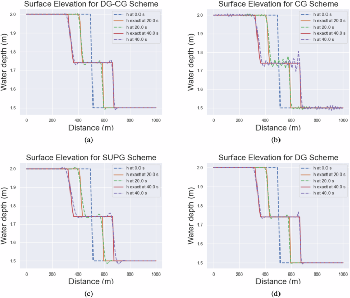
The water height along the x-axis at t = 0, 20, 40 s for all schemes. a solution from DG-CG scheme, (b) solution from standard CG scheme, (c) solution from SUPG scheme, (d) solution from DG scheme.

Full size image

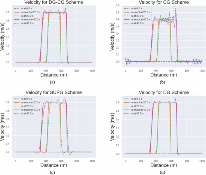
The water velocity along the x-axis at t = 0, 20, 40 s for all schemes. a solution from DG-CG scheme, (b) solution from CG scheme, (c) solution from SUPG scheme, (d) solution from DG scheme.

Full size image

Wetting and drying

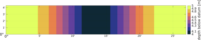
This test case demonstrates SWEMniCS’ capability of handling wetting and drying by adapting the α scheme of Kärna⁴⁶ to work with the DG scheme described in (22). The test case comes originally from an inter-comparison paper by Balzano⁴⁷ and subsequently used for testing in ref. ⁴⁶. The domain is a rectangle that is 13,800 m in the x direction and 7200 m in the y direction. The rectangle is discretized uniformly by 144 triangular elements that have lengths 1150 m in the x direction and 1200 m in the y direction, as in Fig. 5. The bathymetry is a uniformly sloping beach in the x direction that begins 5m below the geoid at x = 0 and ends at 0 m relative to the geoid at x = 13,800 m. The initial conditions are set so that the water is flat at the geoid ζ(x, y, 0) = 0 m and still (u(x, y, 0) = v(x, y, 0) = 0m/s). The left boundary is set as an open boundary that is harmonic in time with an amplitude of 2 m and period of 12 h. All other boundaries are set as wall conditions. The simulation is run from t = 0 days until t = 7 days. The Manning’s formula as in (19) is used for the bottom friction term and the coefficient is uniform in the domain with a value of 0.02 s/m^1/3. Elevations and velocities are recorded over time at three stations along a cross-section within the domain as shown in Fig. 5 at x = 9000 m, x = 11,000 m, and x = 13,500 m.

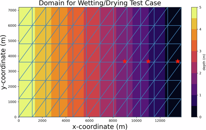
The recording stations are marked with stars, the bathymetry contours are plotted in color. The left-hand side of the domain begins at a depth of 5 m while the right-hand side has a depth of 0 m. The open boundary that forces the tides is on the left side.

Full size image

SWEMniCS is run with a time step of 600 s with the DG formulation of (22) modified for the wetting and drying scheme described in section “Wetting and drying” with α = 0.36. Furthermore, SWEMniCS is run both with the conservative and non-conservative versions of the momentum equations. In order to compare the results from SWEMniCS, the extensively validated SWE model, ADCIRC, is also run for this case but with a time step of 60s due to CFL constraints.

Figures 6–8 show the timeseries of the surface elevations and water velocities at each of the three stations at x = 9000 m, x = 11,000 m, and x = 13,500 m respectively. Across all three figures, we can see that the difference in results for water depth between the two SWEMniCS configurations is minimal, with a root mean square difference of 9.984 × 10⁻⁴m between conservative and non-conservative momentum formulations. As the stations get closer to the right of the domain, we do see differences in the velocity profiles between the SWEMniCS configurations. In particular, we can see that in the rightmost station of Fig. 8, the root mean square difference in the velocities is 7.583 × 10⁻³m/s. The differences in the other two stations were less at 5.61209 × 10⁻³m/s and 4.84593 × 10⁻³m/s. In terms of computational performance, it was observed that the usage of the non-conservative momentum equations resulted in an approximately 27 percent faster run time than the conservative momentum equations. This was because the Newton solver converged with a quarter less iterations on average with the non-conservative momentum equations than with the conservative. Additionally, it was observed that the conservative formulation failed to converge to a solution with time steps larger than 600 s while the non-conservative formulation was able to converge to a solution at time steps as large as 3600 s. This is likely owed to the fact that the formulation with the non-conservative momentum equations reduces the amount of nonlinearity in the problem as seen in “Wetting and drying” section.

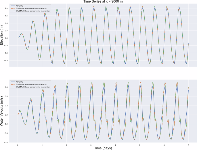
The resulting water depths and velocities for the wet/dry case at the left-most recording station. The water at this point nearly becomes dry.

Full size image

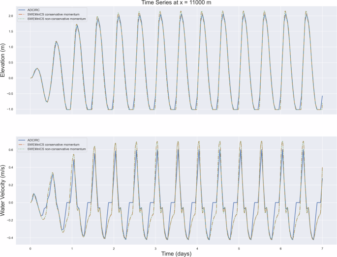
The resulting water depths and velocities for the wet/dry case at the middle recording station. The water at this point does change from wet to dry over the course of the simulation.

Full size image

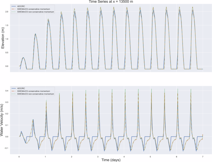
The resulting water depths and velocities for the wet/dry case at the right-most recording station. The water at this point does change from wet to dry over the course of the simulation and spends considerable time in a dry state.

Full size image

When comparing the SWEMniCS results to ADCIRC, the timing of the wetting and the drying at each station appear to be in agreement at all stations. In Fig. 8, we can see that the max water elevations for SWEMniCS are  ≈ 0.1 m higher than ADCIRC. This could be due to the required presence of viscosity within the ADCIRC formulation as well as from damping due to ADCIRC’s wetting and drying. The differences in the velocity values as a particular station becomes dry are likely due to the fact that ADCIRC’s scheme involves activating/deactivating elements depending on their wet or dry state while SWEMniCS operates more like a minimal depth algorithm that always computes a velocity. Despite this, the timings of the maximum/minimum velocities at each station match and the maximum values are all within 7 percent at the leftmost two stations. For the rightmost station, the difference in maximum velocities is approximately 30 percent for the conservative SWEMniCS scheme and ADCIRC while it is approximately 40 percent for the non-conservative SWEMniCS and ADCIRC. This is likely due to a combination of the required inclusion of viscosity in ADCIRC as well as the differences in the wetting/drying scheme.

Hurricane test case

To verify that our models can accurately reproduce real-world physics, we implement a simulation of Hurricane Ike (2008), which peaked as a category 4 storm in the open ocean, and made landfall as a category 2 storm near Galveston, Texas⁷. Hurricane Ike generated peak storm surges of over 5 m and is of particular interest due to the availability of observational data⁴⁸. The mesh used was originally developed for testing ADCIRC, and contains 58,369 triangular elements, see Fig. 9. It covers the entirety of the Gulf of Mexico, as well as the eastern coast of the United States. Mesh resolution is variable with the greatest detail near the coast. Floodplains are not included and the coastal boundary is treated as a wall. Future work will investigate the use of the SWEMniCS model with operational-grade meshes which include detailed floodplains. Such meshes typically have millions of elements and represent the gold standard in hurricane modeling⁷.

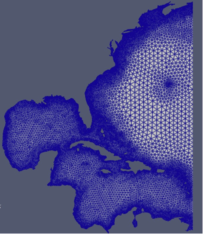
The mesh is fully unstructured and comprised of 58,369 triangular elements. The mesh is designed so that the element size decreases as the coastline is approached from the Atlantic Ocean or Gulf of Mexico.

Full size image

Due to the size of the physical domain, the numerical schemes must solve the spherically projected shallow water equations as in “Spherical Coordinates” section. For both tidal boundary conditions and the tidal potential forcing term, eight tidal constituents are used (M2, S2, N2, K2, K1, O1, P1, and Q1). Finally, we use Oceanweather Inc. (OWI) meteorological forcing data for Hurricane Ike⁴⁹. The data has a spatial resolution of one-tenth of a degree and a temporal resolution of 15 min over 8.5 days. Despite the lack of wetting and drying, this simulation represents a thorough test of the scalability and physical modeling capabilities of our software.

Quantitative validation is provided by comparing our predicted results to observational data at several locations on the coast. Because the mesh does not contain rivers or a significant inland floodplain, much of the available observational data for Hurricane Ike is not applicable. However, we do include a comparison with ADCIRC on the same mesh, to help differentiate between errors in our physical parameterizations and those arising from the limited mesh resolution. The inclusion of ADCIRC also enables us to assess the speed of our shallow water solvers, developed using a general-purpose Python framework, to an optimized, Fortran implementation. We have additionally included video of the Hurricane Ike simulation in the online supplemental material, which provides a further, albeit qualitative validation of our model.

From our extensive numerical testing, we observe that the DG scheme from section “DG Finite Elements” performs the best for this test case and therefore presents only results using the DG scheme in this section. A highly attractive feature of the FEniCSx framework is its built-in MPI parallelism. Assembly of the stiffness matrices is done in parallel by FEniCSx, and the solution of linear systems is handled by PETSc. We observe excellent scaling results for the Hurricane Ike simulation up to 32 processors in Fig. 10.

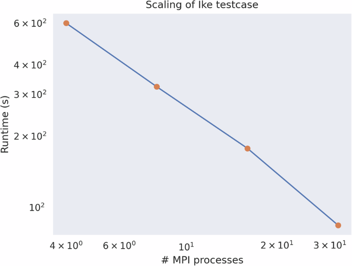
The plot compares MPI processes to overall run time. Ideal scaling was observed up until 30 processes, at which point communication overhead limits performance.

Full size image

A major motivation for using an implicit time scheme is the ability to take large timesteps. We find that in this case the timestep can be increased up to 3600 s without adverse impacts on physical accuracy or numerical stability. Although our implementation is stable for larger timesteps, further increasing the timestep causes the tidal signal to be under-resolved. While larger timesteps reduce the overall simulation time, the relationship is not linear, as demonstrated in Fig. 11. Increasing the timestep also results in more poorly conditioned linear systems during the Newton iteration, which therefore requires more iterations to solve.

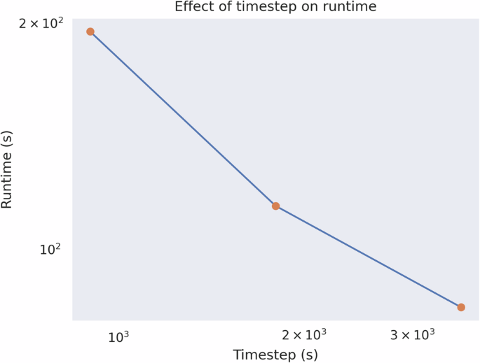
Runtime decreases up until the timestep size of 3600 s. At that point, the underlying Newton solver has difficulty converging from one point in time to the next.

Full size image

Between NOAA tidal gauges and other temporary gauges deployed during Hurricane Ike, we are able to obtain observations of water levels at nine locations that lie within the computational domain. In Fig. 12, we plot the hydrographs of our SWEMniCS implementation relative to an ADCIRC simulation run on the same mesh against observational data. Our model attains roughly equivalent accuracy as ADCIRC does. There is a trend towards underprediction of the peak water levels; as these simulations were carried out on a limited-resolution mesh, these results are unsurprising. The main takeaway is that SWEMniCS is capable of carrying out physically realistic simulations.

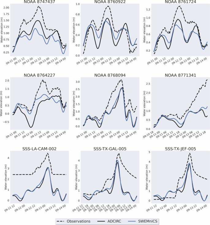
The water surface elevation from nine NOAA gauges that were recorded during Ike is plotted in the dashed lines. The water surface elevations from ADCIRC are plotted with black solid lines, and the water surface elevations from SWEMniCS are plotted with blue solid lines.

Full size image

When using the quadratic friction parameter for SWEMniCS from section “Bottom Friction”, a timestep of 3600 s, and 32 MPI processes, the simulation completes in 90 s. In comparison, the ADCIRC simulation uses a timestep of 6 s and completes in 141 s with 32 MPI processes. Increasing the ADCIRC time step further results in numerical instabilities. Visually, the produced maximum elevation profiles are similar (Fig. 13).

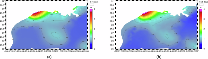
a The maximum surface elevations from the ADCIRC simulation. b The maximum surface elevations from the SWEMniCS simulation.

Full size image

We have introduced a scalable, open-source finite element solver for the SWE within Python based on the FEniCSx library: SWEMniCS. The solver currently contains multiple novel FE schemes including an SUPG-based scheme similar to ref. ¹⁶, a DG scheme with Lax-Friedrichs flux, and an experimental combined DG-CG scheme. All schemes use fully implicit time-stepping schemes based on a generalized BDF2 formula. The resulting nonlinear solver uses the Newton method, taking advantage of FEniCSx’ ability to perform symbolic differentiation.

The solver was tested against several test cases that included a simple case with an analytic solution, a modified lake-at-rest, a dam break, a wetting and drying test case, and a simulation of Hurricane Ike. Expected convergence rates toward the analytic solution with respect to h refinement and p enrichment for all schemes were shown. All three numerical schemes were shown to be well-balanced and capable of accounting for on-grid rainfall. Each of the stabilized schemes showed the ability to handle discontinuities by reducing oscillations in the solution. It was demonstrated that the DG scheme can handle wetting and drying cases via the α scheme of ref. ⁴⁶, with either fully conservative momentum or non-conservative momentum equations. Lastly, the DG scheme showed promising scalability as well as stability and fidelity while taking very large time steps when simulating Hurricane Ike in the Gulf of Mexico. Notably, the SWEMniCS model was able to produce results using a time step of 3600 s while ADCIRC required a time step of 6 seconds to remain stable.

A near-term goal is testing the SWEMniCS model on even larger test cases involving wetting and drying. Future work includes investigation into better preconditioners, as well as inclusion of other finite element schemes such as Hybridized DG or discontinuous Petrov-Galerkin (DPG)⁵⁰ schemes, and inclusion of explicit or semi-implicit time-stepping schemes. Because this code is written in Python, it could also be a useful tool in exploring novel techniques in inverse problems using e.g., ref. ⁵¹, uncertainty quantification, or even augmentation with machine learning libraries and techniques e.g., ref. ⁵² because there can be direct access to the derivatives of the operators within SWEMniCS via FEniCSx support for automatic differentiation.

The 2D depth-integrated SWE arises as a consequence of significantly larger horizontal wavelength scales than vertical, a hydrostatic pressure distribution in the water column, and application of boundary conditions on the sea floor and surface. This leads to a modification of the compressive Navier-Stokes equations and can be found in, e.g., the famous text of Vreugdenhil³. In this section, we present the forms of the SWE that are used throughout within SWEMniCS, as well as some key physics and their parameterizations, and finally, the finite element methods used.

Conservative form

The conservative 2D depth-integrated SWE on a Cartesian coordinate system can be defined as follows²². The specific form is chosen so that any resulting DG finite element schemes are well-balanced in the presence of discontinuous bathymetry.:

H, u, v are the primitive dependent variables which are respectively water depth, depth-averaged velocity in the x-coordinate, and depth-averaged velocity in the y-coordinate. We define ζ = H − h_b as the water surface elevation relative to some fixed geoid, h_b the bathymetry of the land surface that remains fixed in time, g as the constant of gravitational acceleration, τ_B the bottom friction factor, f the Coriolis parameter, C_D the water surface drag coefficient, ρ_water the reference density of water, ρ_air the reference density of air, ({bf{w}}={({w}_{x},{w}_{y})}^{T}) the wind velocity vector, and (frac{partial P}{partial x},frac{partial P}{partial y}) as the atmospheric pressure gradient. Note that (6) can be rewritten more concisely if we define a tensor for the flux, F(U), and write the primitive variables as the vector U = (H, u, v)^T:

where Q = (H, uH, vH)^T is the vector of conserved variables, ∂_tQ denotes time derivatives of the components of Q, and (div({bf{F}}):= frac{partial {{bf{F}}}_{{bf{ij}}}}{partial {x}_{j}}). F(U) comes directly from (6):

with forcing vector f(U):

We will also use the definition of a residual, R, that can compactly be written if given a definition of the relevant shallow water variables, Q, F, f:

Non-conservative form

When working with continuous finite elements as well as with wetting and drying algorithms, the non-conservative form of the SWE may have more favorable numerical properties. This formulation is not valid in the presence of discontinuities. The non-conservative form may be obtained from the conservative form by applying the chain rule along with some algebraic manipulations. There are several works which carefully derive the non-conservative form of the shallow water equations^3,4. We may write the non-conservative form of the SWE as:

where the tensors are defined as:

and f is defined in (9). The non-conservative forms of the SWE will be used in both the SUPG formulation in (20) and in the momentum equations for one of the options with the wetting and drying scheme in (29).

Spherical coordinates

In many practical applications where larger spatial domains are considered, the SWE needs to be solved in spherical coordinates. Within this paper, we will employ projected spherical coordinates to simulate the storm surge from Hurricane Ike. Because FEniCSx allows for specification of the PDE using symbolic notation, we are able to include both the SWE in full spherical coordinates as well as projected spherical coordinates. For the SWE using projected spherical coordinates, we use the equirectangular projection formulation similar to refs. ^15,16,53. Here we denote latitude by ϕ and longitude by λ. A reference coordinate, denoted (ϕ_o, λ_o), is selected and is assumed to be central in the given domain. We define R to be the radius of the earth in meters. The equations are solved in Cartesian coordinates (x, y) and the coordinates are transformed from the original spherical coordinates (λ, ϕ) via:

The flux tensor written for Cartesian coordinates in (8), becomes:

The forcing vector written in (9) for Cartesian coordinates now becomes:

The residual for the strong form of the conservative SWE in spherical projected coordinates can be written compactly as:

Bottom friction

The specific form of the bottom friction term, τ_B, is important in determining the final closed form of the SWE which is all defined via constitutive laws. We currently have three implementations: a linear drag law, a quadratic drag law, and a Manning’s law. The linear friction law can be written as:

where a typical value of the constant c_f = 0.03. The quadratic law can be written as:

As in ref. ²², an example value is 0.003. Lastly, the Manning’s law can be written as:

where g is the acceleration of gravity, and n is the Manning’s roughness coefficient which depends on the material of the land surface. In SI units, Manning’s n can vary from 0.01 to 0.07 m^−1/3/s.

In the next three sub-sections, we present our currently available finite element schemes defined for the SWE.

CG finite elements with SUPG stabilization

The SWE is a hyperbolic system of equations, so it is necessary to utilize techniques that provide numerical stability in order to use continuous finite elements effectively. The SUPG method⁵⁴ is a popular method and has been used for solving SWE in multiple cases^55,56,57. For the test cases presented in the next section, we will use the SUPG formulation from the AdH¹⁶. It is noted that the following numerical scheme will be identical to that of¹⁶ but with one main exception that is the nonlinear solver in SWEMniCS, described in the section “Time Stepping”, utilizes an exact Newton method while AdH uses a finite difference approximation of the Newton method.

To briefly summarize, we begin with the standard Galerkin form which arises from multiplying by a test function p for each of the three equations, integrating across the domain, and then integrating by parts the term containing the flux tensor F. The SUPG term is added to the standard Galerkin form and is a product of the strong form of the residual with the derivative of the test function in the upwind direction. We only consider the SUPG additions in the discrete setting so that these terms are added on an elemental basis. In general, the SUPG weak form for the conservative SWE can be written the following way. Find U ∈ U^h or find Q ∈ Q^h:

where n is the unit normal vector pointing outward, τ_i is a 3x3 matrix for each i (i is defined for each spatial dimension, which in this case is two) that contains the coefficients for the SUPG term, ⊙ is elementwise matrix-matrix multiplication, and R is usually the conservative form of the residual³⁰. It is most common to take the conserved variable Q as the solution in which case ({{bf{A}}}_{{bf{i}}}=frac{partial {{bf{F}}}_{:,i}}{{bf{partial Q}}}) ^55,57. Although this more standard formulation is available in our software, we observed better runtimes with the formulation from AdH and therefore elected to use it for the test cases in the next section.

In the AdH formulation, the primitives U are the solution variable, and the residual term in the SUPG term is in non-conservative form: R = R_nc. As a result, A_i in (20) is A₁ and A₂ from (12). It is noted that there has also been successful usage of the SUPG with the primitives, U, as the solution variable in other equations besides SWE^58,59.

We use the following definition of the stabilization parameter τ_i from¹⁶:

where A_e is the radius of the element, and α is a positive constant typically chosen to be between 0 and 0.5.

DG finite elements

In DG finite element methods, the solutions are allowed to be discontinuous at element interfaces and are continuous in a weak sense. In order for a closed system of equations to be formed, a unique flux must be specified at the element interfaces. DG methods have been used extensively to solve many conservation laws, including the SWE^{22,24,26,60,61,62}. However, the vast majority of these methods with a few exceptions^24,62 use fully explicit time integration schemes that require a CFL constraint in order to preserve stability. The following scheme available within SWEMniCS is fully implicit in time and uses an exact Newton method which is described in Section 4.9. The weak form is: Find U ∈ U^h or find Q ∈ Q^h:

where (hat{{bf{F}}}) denotes the numerical flux. For the flux on the element boundary, we choose to use Lax-Friedrichs upwinding defined as:

In this case, ⁺ denotes the function value on one side of an inter-element edge ∂Ω_e while ⁻ denotes the value on the opposite side of that edge. The average and jump operators are defined respectively as (,text{avg},(cdot )=frac{1}{2}({cdot }^{+}+{cdot }^{-})) and jump( ⋅ ) = ⋅ ⁺ − ⋅ ⁻. The value λ comes from the eigenvalues of the Jacobian of the flux tensor and is defined as:

It is most common to use the conserved variables, Q, as the solution variable with the DG approach as this approach keeps terms that are differentiated by time linear. This allows for the discretized finite element system to be cast more readily into a system of ODE’s to be solved forward in time. Our code allows for the choice of either the solution variable to be the primitives, U or the conserved variables Q. The usage of this DG scheme along with the fully implicit BDF2 time step scheme and exact Newton solver described in section “Time Stepping” has not been implemented before to the best knowledge of the authors. In SWEMniCS, this DG scheme also can handle wetting and drying as described in section “Wetting and drying”.

DG-CG

To demonstrate the flexibility of our software, we have also employed a novel combined FE method where we use a discontinuous finite element method for the continuity equation and a continuous finite element method for the momentum equations. The motivation here is to take advantage of the ability of the DG scheme to capture shocks and maintain local conservation with respect to mass while also reducing the total number of degrees of freedom by using a CG scheme for the two momentum equations.

The scheme is essentially the DG scheme from section “DG finite elements” but with CG solution/test space for the momentum equations. Hence, in the momentum equations there is no numerical flux applied. Here we will note that our finite element space is now a combined finite element space where U ∈ U represents a vector function of length three where the first component is a DG finite element function, and the second and third components are CG finite element functions: U = (H_dg, u_cg, v_cg). This implies that Q = (H_dg, H_dgu_cg, H_dgv_cg). Additionally, the test functions come from the combined space so we will denote p = (p₁, p₂, p₃) where p₁ comes from the DG finite element space and p₂, p₃ comes from the CG finite element space.

The combined formulation is in fact identical to the DG formulation (22) but applied to the combined space. The only simplification is that the inter-element Lax-Friedrichs flux is trivially zero for the two momentum equations because the jump of the now continuous test functions, p₁, p₂, for the momentum equations are trivially zero. Formal analysis of the properties of this scheme is a work in progress, but for the purposes of this research, it is intended as a proof of concept of how simple it is to create new finite element schemes within our FEniCSx based software.

Boundary conditions

All of the finite element schemes described require weak or strong enforcement of boundary conditions. The available boundary conditions currently in the software that will be used in the test cases include open boundaries, and wall boundaries which will both be enforced weakly. For a discussion on which boundary conditions are appropriate for a given problem, we refer to ref. ³ and only state the types of boundaries here.

The open boundary condition is defined by enforcing a Dirichlet condition weakly on the water depth, H = H_o, while leaving the velocities free. This type of boundary arises when tidal heights are used as a forcing function onto a domain. The wall boundary condition is designed to behave as an impenetrable barrier and is implemented by setting the flux normal to the boundary to zero. In our software, the wall boundary condition is enforced weakly. For the CG finite elements, both the wall and open boundaries are accomplished by modifying the definition of F on the appropriate segment of the boundary. If we assume u ⋅ n = 0 on any wall boundary then it must be true that the only non-zero components in F are:

Similarly, for weak enforcement of the open boundary, we replace the definition of F(U) on the open boundary with F(U_o). Where ({{bf{U}}}_{{bf{o}}}={({H}_{o},u,v)}^{T}) are the primitive variables but with the depth variable replaced with the Dirichlet condition for H on the open boundary. For the DG finite elements, we use the standard weak boundary enforcement for walls and open boundaries as described in ref. ²².

Time stepping

The finite element schemes in Sections “CG finite elements with SUPG stabilization”, “DG finite elements”, and “DG-CG” are all written in semi-discrete form. In order to have a fully discrete system, the temporal derivative is approximated via finite difference. Currently, the implemented time stepping scheme is the fully implicit generalized BDF2 as in ref. ¹⁶. The fully implicit time-stepping scheme allows for SWEMniCS to take larger time steps than the typical CFL constraints of explicit time-stepping schemes^5,26,61 and could therefore bring potential performance benefits when the CFL condition is particularly restrictive. The scheme operating on flux Q is defined as:

The time step size is defined as Δt, with n being an integer that represents the nth discrete time level, and the parameter α is a scalar constant that can vary between zero and one. A value of α = 0 would result in the first-order implicit Euler scheme while a value of α = 1 would result in the second-order BDF2 scheme. This scheme is fully implicit, meaning all of the terms outside of the finite difference approximation to the time derivative are evaluated at time level n + 1. This results in a nonlinear system of equations at each time step that is solved via Newton’s method. An advantage of using the FEniCSx software is that it is capable of automatically computing the Jacobian necessary to define the Newton method via symbolic differentiation. The underlying linear solver uses the PETSc library and by default uses the GMRES iterative solver with block Jacobi preconditioning.

Wetting and drying

In many practical applications, the domain of interest may include areas that transition between wet (H > 0) or dry (H = 0) over the course of a simulation. The SWE becomes ill-defined as H → 0 and so in practice an empirical treatment must be used in order to allow for wetting and drying. In SWEMniCS, we adapt the α scheme of Kärna⁴⁶ so that it is compatible with the finite element and time-stepping schemes from the previous sections. This scheme was chosen because it is designed to work with implicit time-stepping schemes (no required time-step restriction) and it is convenient to implement within the FEniCSx library because it can be directly written in Unified Form Language. For the purposes of this study, the α scheme is only applied to the DG scheme from section “DG finite elements” although the application of the α scheme towards the SUPG-based scheme is planned future work.

The main idea of the α scheme is to introduce a special function f(H) to enforce positive water depths. This can be interpreted as allowing for the bathymetry to move over time to enforce a very small minimal depth. For more details on the α scheme, readers are referred to ref. ⁴⁶.

The α scheme is applied to the scheme in section “DG finite elements” by replacing any instances of the variables within U with (tilde{{bf{U}}}={(tilde{H},u,v)}^{T}), Q with (tilde{{bf{Q}}}={(tilde{H},utilde{H},vtilde{H})}^{T}), and h_b with (tilde{{h}_{b}}). The modified variable, (tilde{H}), is defined by adding the aforementioned function f(H) so that (tilde{H}) must always be positive. The definitions for (tilde{H}), (tilde{{h}_{b}}) along with the choice for f(H) in SWEMniCS (same as in ref. ⁴⁶) are:

It is noted that the choice for f(H) is arbitrary so long as: (tilde{H} > 0) for any H, f(H) ≈ − H as H decreases below 0, f(H) ≈ 0 as H increases above 0, and f(H) must be continuously differentiable for any H. An appropriate choice of α is one that is as small as possible but must grow with the change in bathymetry from one element to the other. It is noted that even though (tilde{H}) is replaced into the FE formulation, the solution variable remains H (therefore allowing for negative H). One convenient property of this scheme is that the water surface elevation from the solution remains unchanged regardless of the swapped variables: (zeta =H-{h}_{b}=tilde{H}-tilde{{h}_{b}}).

The test case in section “Wetting and drying” demonstrates the usage of the α scheme within SWEMniCS for both a conservative and non-conservative form of momentum equations. The FE form with wetting-drying for the conservative momentum equations is identical to the FE form without wetting-drying from section “DG finite elements” except for two modifications: the first is the replacement of any occurrences of H or h_b with the positivity-enforcing (tilde{H}) and (tilde{{h}_{b}}) from (27), and the second being a slight manipulation of the definition of the flux tensor F to minimize the number of occurrences of the nonlinear additions to (tilde{H}) and (tilde{{h}_{b}}). We note that this modification is exact in the formal setting but practically will reduce the number of occurrences of the computation of the nonlinear function f(H) in the weak form due to the fact that ζ doesn’t require the usage of f(H). The new flux definition with wetting and drying can be written as:

We can see that the manipulation in (28) to the form on the right side makes the flux only linearly dependent on the positivity-enforcing function f(H) while also reducing the total number of occurrences of f(H) in the definition of F.

Within SWEMniCS, we also allow for the usage of the DG scheme with wetting and drying for the non-conservative momentum equations as in section “Non-conservative form” (still using conservative form of continuity equation). The motivation for including this is two-fold. First, it is to compare results from cases involving wetting and drying with the fully conservative momentum equations. The combination of the usage of the conservative continuity equation and the non-conservative momentum equations is the same as what the α wetting and drying scheme was originally applied to in Kärna⁴⁶. The main difference with its usage in SWEMniCS is the choice of numerical flux and time step scheme.

Second, the usage of the non-conservative momentum equations eliminates any definition of (tilde{H}) or (tilde{{h}_{b}}) outside of the potential usage within the source term. This could improve computational performance of SWEMniCS by reducing the amount of nonlinearity present in the conservative momentum equations.

The application of the α scheme to the conservative continuity equations and non-conservative momentum equations to the FE scheme in section “DG finite elements” can be written in the following way. Find U ∈ U^h:

Here, u = (u, v)^T is just the velocity components from the solution, p_m = (p2, p3)^T are the test functions for the x and y momentum equations. F_c is the flux tensor as in (28) but with the second and third rows containing the gravity terms from the non-conservative momentum equations as in (11). The source term also changes from the previous definition because we elect to move all gravity terms within the flux tensor to avoid extra definitions of the nonlinear f(H). F_c and f_* are defined as:

We employ the same numerical flux as in (23) to uniquely define any variables on the interface. We can see now that this non-conservative formulation does not include any usage of f(H) within the flux terms or time derivatives of the momentum equations.

Results involving wetting and drying from the fully conservative scheme and the non-conservative momentum scheme will be compared in section “Wetting and drying” against a validated SWE model ADCIRC.

Additional details

Mixed order p elements are allowed, meaning that for any weak form mentioned above, we can select a different polynomial order for each solution variable. However, in all of our test cases, we use uniform-order polynomials. Although any appropriate element type is allowable in FEniCSx, for the test cases described below we simply use Lagrange elements defined on triangles.

To ensure that SWEMniCS can be a potentially competitive alternative to existing software and moreover can access high-quality inputs from ADCIRC, SWEMniCS is supplied with conversion scripts for ADCIRC inputs.