The 11-month precursory fault activation of the 2019 ML 5.6 earthquake in the Weiyuan shale gas field, China
Introduction
In recent years, subsurface injection activities, including hydraulic fracturing, have been cited as the leading cause of rising seismicity in regions that were historically quiescent1. Hydraulic fracturing, an advanced technology applied in the shale oil & gas industry, enhances oil & gas recovery by injecting high-pressure fluids in low-permeability shale to stimulate fracture growth2. Although the fracturing process was originally considered to cause microseismicity with magnitudes below zero, unexpected events with higher magnitudes were reported to accompany HF operations3,4. By far, HF-triggered earthquakes of increasing magnitudes, up to Mw 5.4, have been documented at many locations around the world5,6,7,8,9. Because such faults are largely unknown until an earthquake occurs, there has been no effective monitoring of fault activation to assess how large an earthquake might strike.
Many physical mechanisms have been proposed to explain induced seismicity, including pore pressure diffusion10, poroelasticity effect11,12, aseismic slip13,14, and inter-event stress transfer15. In practice, the scenario can be complex, as the triggering of an earthquake can be the combined work of multiple mechanisms. Understanding these intricacies is hindered by the lack of near-fault observations so that detailed triggering processes of destructive earthquakes were rarely thoroughly recorded. As this precursory phase can span many months, utilizing the data in this period is crucial for hazard assessment.
Furthermore, delayed triggering of earthquakes after injection ceased has been widely observed, which complicates the design of an effective risk mitigation strategy. In many cases, the largest events occur near or after well completion in days to weeks2,16,17,18,19,20,21. Whether these earthquakes are directly related to injection and what physical mechanisms are responsible remain elusive. To compound the problem, there could be multiple wells that are stimulated at different times in close spatial proximity to each other, and they can all play a role in bringing the fault system closer to failure with each successive stimulation. Thus, observing how the fault is activated by injection operations over time is key to effective risk mitigation.
All of the above challenges in risk monitoring are present for induced seismicity in the Weiyuan shale gas field in Sichuan, China. In particular, the ML 5.6 earthquake that struck in September 2019, causing much economic damage and casualties22, occurred with very little warning on a previously unknown fault, more than 3 months after injection shut-in. In this work, we present detailed observations of the long-term preparation process of the 2019 Weiyuan ML 5.6 earthquake assisted by near-fault stations (Fig. 1A). We report large-scale activation on the main fault plane, which started ~11 months before the mainshock, coinciding with fluid injection from an HF well pad whose wells intersected the fault plane. Another HF operation in a nearby well 6 months later. After this, there was a 3-month period of relative seismic quiescence, before the sudden rupture of the ML 5.6 earthquake. To understand the triggering mechanisms, we set up a numerical model with a fault in 2D antiplane shear in a homogeneous elastic medium, governed by rate-and-state friction and coupled to pore pressure diffusion from fluid injection. Our simulations show that post-injection aseismic slip events over multiple injection operations could explain the delayed triggering of the ML 5.6 earthquake. This study advances our understanding of HF-triggered earthquakes, suggesting the importance of long-term observations for earthquake preparation and taking into account post-injection aseismic slip.

A Map view showing the ML 5.6 epicenter and the focal mechanism, local structures and earthquakes before the ML 5.6 event since 2015. The inset shows locations of historical (1972-2012) ML > 4.5 earthquakes in light blue dots (https://data.earthquake.cn) in and around the Sichuan Basin with GPS velocities field84, and active faults (blue). The red star is the ML 5.6 epicenter. B Zoomed-in view of the dashed box in (A). The coseismic deformation area29 is shown in a gradient of blue in the enclosed region. 14-day aftershock distribution of the ML 5.6 earthquake and adjacent well pads are plotted. Red lines stand for fault traces at shallow depth according to aftershock distribution. The fault consists of the main fault patches P1, P2 and a secondary patch P3. Black dashed lines represent buried depths of the target shale layer. C Along-strike cross-section view showing aftershocks with strata information and projection of vertical wells of adjacent well pads. H04 and H37 do not intersect the fault and are plotted in dashed lines. Aftershocks form an elliptical distribution, and the ML 5.6 hypocenter is marked by a red star.
Results
Background
The ML 5.6 (Mw 5.0) Weiyuan earthquake struck on 8 September 2019 in the WSGF. The event is among the largest HF-triggered earthquakes globally and led to 1 death and 63 injuries. To the northwest of the WSGF lies the current inactive Weiyuan anticline, the historical structural deformation of which led to gentle southeastern-dipping strata distribution (Fig. 1A). The target shale layer is located at the bottom of the Silurian shale strata (shale-rich strata I) with buried depths of 3.0–3.5 km in the study area23 (Fig. 1B). Strata between the shale-rich strata I to the pre-Ediacaran basement present a “sandwich” structure with the ~460 m thick Lower Cambrian shale (shale-rich strata II) embedded in the dolomite-rich strata (Fig. 1C). The ML 5.6 hypocenter is located in the Ediacaran dolomite strata that lie below the shale-rich strata II. The pre-Ediacaran basement is composed of volcanic debris sediments and granite24.
Historically, the seismicity rate at the WSGF was low, with no occurrence of ML > 4.5 events within 50 km of the ML 5.6 epicenter before 2012 (with historical records since 1972), when the WSGF was established. Massive HF operations began in mid-2015 and led to a surge in earthquakes21. Injections close to the ML 5.6 epicenter were carried out in the well pads H04 in 2015, H39 in 2018, and H37 in 2019 (Fig. 1B). In the H39 well pad, which intersects the traces of the ML 5.6 fault patch, casing deformation with shear slip up to 1.61 cm was reported25 (Fig. S1). Apart from HF operations, there were salt mining activities in Zigong city and waster-waster disposal inside the Weiyuan anticline. However, these sites are more than 20 km away from the ML 5.6 epicenter and should play a minimal role compared to HF injections.
Earthquake relocation
To understand the mechanisms of the Weiyuan ML 5.6 earthquake, we first constructed an earthquake catalog using near-fault stations, which became available since March 2019. Four of these stations are within 6 km of the ML 5.6 epicenter (Fig. 1B). We started from the catalog reported by the Sichuan Earthquake Agency (SEA) and refined picked P&S arrivals. We then computed optimal velocity models (Fig. S2) incorporating borehole measurements and conducted absolute earthquake location using the six closest stations that are most sensitive. The locations were then refined by the double-difference relocation algorithm, hypoDD26, with P&S wave cross-correlation differential times included (Table S1). Later, template matching was conducted to enhance the catalog (see Methods). The utilization of near-fault stations and velocity models originated from borehole measurements led to a high-resolution earthquake catalog with small relative location errors (horizontal and vertical errors of 9.8 m and 8.6 m, respectively). Consistency was also achieved between aftershock locations and the reported fault identified from seismic reflection profiles27 (Fig. S3). Aftershocks delineated a clear fault geometry with a strike orientation of 40°, dipping to SE at 38° (Figs. 1A, 2D), which can be activated under the approximately E-W orientation of the maximum horizontal compressive stress (({{{{rm{SH}}}}}_{max })) in the study area28. The shallow reverse-faulting event has a right-lateral strike-slip component22, leading to distinct surface deformation with a maximum displacement of ~ 3 cm29 (Fig. 1B).
The earthquake rupture was directed towards the northeast30 along the northeastern-striking fault, which consists of the main fault patches P1 and P2 that extend down-dip toward the basement and a secondary fault patch P3 with limited vertical extension (red lines in Fig. 1B). Intense aftershocks occurred at the top of the shale-rich strata I and the basement (Fig. 1C, Fig. S4B), which bound the vertical range of the mainshock rupture. Such a feature might indicate a geological control on earthquake rupture. Many shallow aftershocks are distributed along P2 and P3, while only a few exist along P1, which experienced intense precursory activation before the ML 5.6 earthquake. Aftershocks in the northeast and southwest denote the lateral extent of the mainshock rupture. We used an ellipse to denote the rupture area in the along-strike section plot (Fig. 1C). The ellipse has a long axis length of 6.6 km and a short axis length of 1.34 km in depth (2.2 km along fault dip), resulting in a rupture area of ~ 11 km2. Aftershocks first enclosed the rupture area and later expanded to a larger area, indicating the potential role of afterslip.
Differences between HF-induced earthquakes and on-fault earthquakes
To characterize features of HF-induced earthquakes and seismicity on the fault that hosted the ML 5.6 earthquake, we conducted hierarchical clustering using S-wave similarity for relocated events. We made use of near-fault stations and employed multiple-station-based hierarchical clustering for 2059 events, including 1188 events before the ML 5.6 earthquake since March 2019 and 871 aftershocks within 14 days after the mainshock (see Methods, Fig. S5). After clustering, we have 1219 events (59% of the total number) grouped into 17 self-similar clusters and 840 unclustered events. Events within a cluster have high waveform similarity coefficient and the coefficient is low for event waveforms in different clusters (Fig. S6). New events detected by template matching are assigned the same cluster IDs as their templates.
Guided by clustering results, we identified two categories of seismicity according to their spatial locations. The first category includes 10 clusters and adjacent earthquakes (cluster IDs 1–10 in zones labeled (1), (2), and (3) in Fig. 2). These events are close to the injection layer and the HF well pads, extending horizontally parallel to the strata (Fig. 2, Fig. S4C). The second category includes 7 clusters and nearby seismicity located on the main fault (cluster IDs 11–17 in Fig. 2). Clusters 11–15 are located in the main fault zone, while 16–17 are two isolated clusters on the shallower and deeper extension of the main fault. We thus infer the two are also on-fault clusters. We use HF-induced earthquakes to refer to seismicity directly associated with HF operations and on-fault earthquakes to represent induced earthquakes that occurred on the main fault.
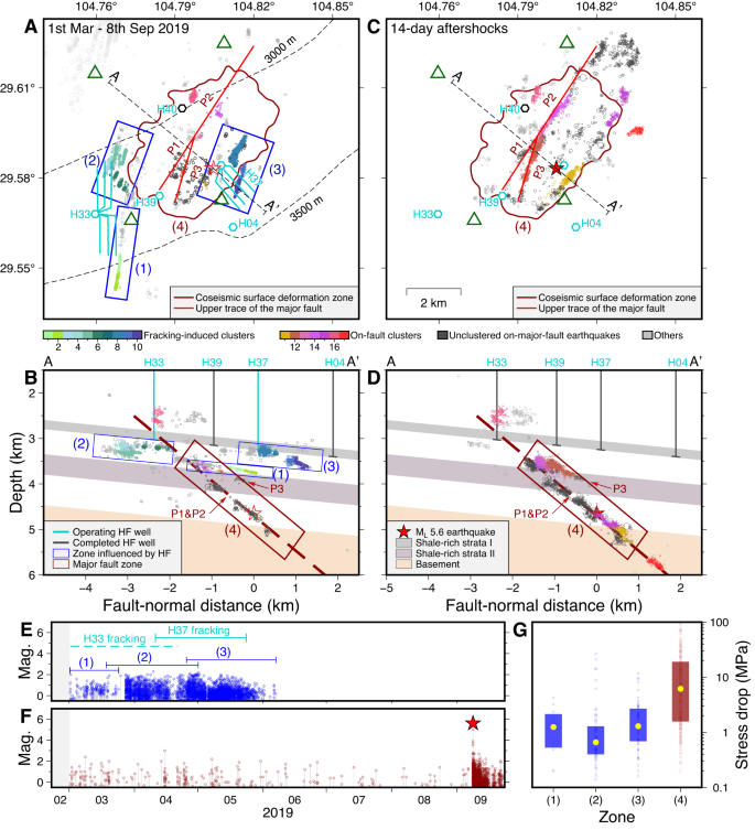
HF-induced clusters and on-fault clusters are colored; unclustered events are in gray. Map and fault-normal views: (A, B) before the ML 5.6 earthquake. Blue boxes enclose HF-induced earthquakes. HF activities were conducted in H33 and H37 during this period; (C, D) after the ML 5.6 earthquake. The dark red box indicates the main fault zone, consistent with the inferred rupture area in Fig. 1C. Three fault patch traces are marked. E Magnitude vs. time plot of HF-induced seismicity in blue boxes from (B). The elapsed time of seismicity in the three zones are labeled (1)–(3). The exact HF duration in H37 is plotted in solid cyan line and inferred HF duration in H33 is plotted in cyan. F Magnitude vs. time plot of seismicity in the main fault zone and aftershocks. G Distribution of reported stress drop values (circles), percentile bars (25–75%), and median values (dots) in zones (1)–(4) for ML 0.5–ML 2.0 events31.
In addition to the differences in spatial distribution, HF-induced earthquakes and on-fault earthquakes are different in three aspects. First, HF-induced clusters and adjacent earthquakes have limited durations that are consistent with the HF period (Fig. 2E). For example, earthquakes in the vicinity of the H37 well pad began 15.4 days after HF started and stopped 13.7 days after shut-in. However, on-fault earthquakes persisted for the entire period from March to September 2019 and mainly occurred on the main fault patches (P1 and P2 in Fig. 2B). Second, HF-induced clusters have a diffusive migration pattern with fitted hydraulic diffusivity up to 0.05 m2/s (Fig. S7). Finally, from Fig. 2G, analysis of stress drop values derived by a new method based on spectral decomposition combined with a global optimization algorithm31 reveal that the median stress drop values of HF-induced earthquakes in zones (1)–(3), which are in the range of 0.66–1.29 MPa, are systematically lower than on-fault earthquakes. For earthquakes in the main fault zone (4), the median stress drop value is 6.17 MPa. For on-fault clusters 16 and 17, the median stress drop is 3.38 MPa. This stress drop contrast should be the consequence of increased pore pressure in HF-induced earthquakes31,32.
As earthquakes in the main fault zone were recorded at the availability of dense near-fault stations (Fig. 2F), it indicates that fault activation started before March 2019. To understand the complete history of fault activation, we conducted double-difference earthquake relocation from January 2015 to February 2019. As seismic network coverage was limited before March 2019, the bootstrap test resulted in median horizontal and vertical location errors of 66 m and 49 m, respectively, higher than in the later period when the array of near-fault stations became available (see Methods). We also conducted template matching for this period to enhance the catalog. A waveform similarity criterion was applied for on-fault earthquake identification to account for both earthquake locations and mechanisms. For a relocated event to be identified as an on-fault earthquake, it should be similar to at least one later (since March 2019) on-fault earthquake with S-wave cross-correlation coefficients greater than 0.7 on at least 3 stations. Comparison with earthquake distribution reveals that identified earthquakes are located in the main fault zone (Fig. S8; Supplementary Movie 1), showing the reliability of the identification.
Multi-stage fault activation
Earthquakes in the main fault zone first appeared in September 2018 and escalated on 14 October 2018 (Fig. 3E), indicating the beginning of fault activation. During the period, HF operations were performed in the H39 well pad. The consistency in time between the HF period and the activation of the fault, the spatial intersection between the well pad and the fault, as well as the large casing deformation reported in the H39 well pad25 lead to the inference that injection in the H39 initiated the fault activation.

Seismicity patterns in the shallow (S) and deep (D) segments of P1 and P2 in 4 stages. Wells of H04, H39, and H37 were projected in section plots (A–D). H33 is outside the display range. A Stage I: with HF from H39. On-fault earthquakes occurred sequentially from (1) to (4) in the shallow segments of P1 and P2. Starting in 2019, the shallow segment of P1 was activated and seismicity extended deeper from (5) to (6). B Stage II: Numerous earthquakes occurred in P1. ML 3.7 and 3.8 events occurred in February 2019. C Stage III: with HF from H37. Earthquakes were mainly in the shallow segment during HF, first on P1 (labeled (1)), then on P2 (labeled (2)). Soon after H37 shut-in, some earthquakes happened near the ML 5.6 hypocenter (labeled (3)). D Stage IV: no HF. Low earthquake occurrence rate. During the last 5 days, events occurred in the deep segment of P1, including an ML 3.5 event 6 min before the mainshock. E Summary of HF operations and on-fault seismicity since 2015. Fault activation started in October 2018. Histograms represent the number of earthquakes on P1 every 2 days. Distance vs. time plot shows the seismicity front (red arrows) advancing toward the ML 5.6 hypocenter.
Before 2018, HF operations were conducted on the H04 well pad in mid-2015. Although earthquakes occurred, they were shallow and were not located in the main fault zone by the identification criteria (Fig. S8A, E, I). Since the seismic network remained unchanged from May 2015 to February 2019, the identification of fault activation is not a biased result due to network change. Furthermore, the absence of seismicity in the main fault zone from 2015 to 2018, when the H04 well pad was in production, indicates that shale gas extraction played a limited role in fault activation.
As the fault began to activate, earthquakes in the main fault zone lasted for 11 months until the ML 5.6 earthquake. We divide the fault into the shallow segment (shale-rich strata II) and the deep segment (dolomite strata), and characterize the fault activation in four stages (Fig. 3A–D). The first stage lasted ~4 months (14 October 2018 to 7 February 2019), during which the H39 well pad experienced HF. Intense seismicity occurred around the H39 well pad, including many earthquakes that took place between shale-rich strata I and II (Fig. S8B, F). These earthquakes indicate the hydraulic connection between the two shale-rich strata. Identified seismicity in the main fault zone first appeared in the shallow segment, which corresponds to the shale-rich strata II, with a sequential occurrence in P1 and P2 (labeled (1)–(3) in Fig. 3A, E). These earthquakes show a migration pattern consistent with a diffusion front with a hydraulic diffusivity of 0.20 m2/s (Fig. S9A), indicating that the initial activation of the fault might be dominated by pore pressure diffusion. The diffusivity is higher than values related to other well pads (Fig. S7), showing a higher permeability of the main fault. Later, an ML 3.5 event occurred in the shallow segment of P2 (labeled (4) in Fig. 3A, E). After that, the number of earthquakes in the main fault zone kept decreasing.
Earthquakes around the northern branch of H33 well pad appeared on 1 January 2019, indicating HF in H33 started (Fig. S8C). These earthquakes extended parallel to the strike of the main fault with a lateral separation of ~2 km (Fig. S8C). In 13 January 2019, three months after the initiation of fault activation, the shallow segment of P1 was reactivated and earthquakes penetrated the deep segment of P1 (labeled (5), (6) in Fig. 3A, E), indicating an aseismic slip front or pore pressure diffusion front that drove the seismicity deeper. The temporal proximity between the start of HF in H33 and the reactivation of the main fault indicates that there might be a causal relationship. If HF in H33 contributed to later earthquakes, it was most likely through poroelastic effects, as it can trigger relatively distant earthquakes in a short time and did not require hydraulic connectivity. Upon the activation of the deep segment of P1, P1 and P2 exhibited distinct evolutionary paths with increasingly more events occurring in the deep segment of P1.
The second stage lasted ~2 months (10 February to 9 April 2019) and ended before HF at H37 (Fig. 3B). An ML 3.7 event on the first day, an ML 3.8 event 4 days later at a shallower depth, and their aftershocks spanned a large region on P1 and moved the seismicity front even closer to the ML 5.6 hypocenter (Fig. 3E). Therefore, Coulomb failure stress transfer dominated fault activation during this stage. Later, the number of earthquakes on P1 started to decline. Continuous earthquakes occurred around the H33 well pad during this stage (Fig. 2E), showing H33 was under HF. However, we did not observe any earthquakes that migrated from H33 to the main fault. This spatial separation is clearly shown in Fig. 2A. Although the H33 well pad experienced injection and HF-induced seismicity during this stage, its impact on the main fault activation should be limited both due to its long distance from the mainshock epicenter (4.7 km) and the absence of earthquakes that connected the HF-induced seismicity to the main fault (red lines in Fig. 2A).
The third stage lasted ~2 months (10 April to 6 June 2019), corresponding to the beginning of HF in H37 until 14 days after HF ended. H37 was located in the hanging wall of the fault and did not directly intersect it (Figs. 1B, 3C). The number of earthquakes in the shallow segment soon increased in P1. Later, a number of earthquakes occurred in the shallow segment of P2, which was relatively inactive in the previous stage (labeled (1), (2) in Fig. 3C, E). Right after well shut-in, trailing seismicity shifted from the shallow segment to the deep segment with the occurrence of a number of earthquakes in the vicinity of the ML 5.6 hypocenter (labeled (3) in Fig. 3C, E). Rapid and distinct depth responses on the fault to HF operations indicate the role of poroelastic effects in this stage.
Finally, the fourth stage corresponds to the final ~3 months before the ML 5.6 mainshock (7 June to 8 September 2019) with no injection operations (Fig. 3D, E). The seismicity rate is low and there is no clear spatiotemporal pattern. In the last 5 days before the ML 5.6 earthquake, several earthquakes appeared close to each other and culminated in an ML 3.5 event, which occurred 6 minutes before the mainshock and exerted a static shear stress transfer of 0.05 MPa (Fig. S10), a value close to the earthquake triggering threshold33.
Aside from the observations above, there exists a long-lasting group of seismicity near the H40 platform (Fig. S8B–D; Fig. 2A, C), including earthquakes in cluster 16. These earthquakes first appeared with the construction of the H40 well pad in 2018 and persisted after the ML 5.6 earthquake. As the H40 well pad did not experience HF before the ML 5.6 earthquake, this seismicity was most likely triggered by well-drilling operations. The observed phenomenon might indicate critical stress levels on faults around the H40 platform.
In summary, our observational work reveals that the 11-month precursory fault activation of the ML 5.6 earthquake is a complex process with a variety of mechanisms from multiple well pads at play. The initial activation occurred in the shallow segment and showed a migration pattern associated with pore pressure diffusion from injection at the H39 well pad. The activation and the mainshock in later stages were dominated by Coulomb failure stress transfer of three ML ≥ 3.5 events, a scenario that resembles natural earthquakes. The poroelasticity effect of H37 was modulated in later stages. Injection-induced aseismic slip likely also played a role during fault activation.
It remains elusive why the ML 3.5 and ML 5.6 earthquakes occurred 3 months after the shut-in of the H37 well pad. Here, we show it’s unlikely that pore pressure diffusion, poroelasticity effect and shale gas extraction are the driving mechanisms. Assuming pore pressure diffusion was present in the later fault activation of the deep segment, we quantified seismicity distribution using a hydraulic diffusivity of 0.05 m2/s, a value much smaller than the estimated main fault diffusivity. The ML 5.6 earthquake did not happen even when the pore pressure front should have reached the hypocentral area (Fig. S9B). Another mechanism that has often been proposed for delayed triggering is poroelastic stressing. However, it often occurs in a short time span, as stress relaxation after injection stops leads to immediate rupture of previously stabilized faults34. Thus, this alone is also not a plausible explanation for the 3-month delay after the shut-in of H37. To examine whether shale gas extraction at the H37 well pad may have impacted earthquake triggering through poroelastic stress transfer, we estimated the net injected mass and volume (injection minus flowback and extraction) in Fig. S11. Overall, the net injected mass and volume are positive, so even though the poroelastic effect is reversed during extraction, it should not have more impact than injection. Therefore, we believe that the long delay is unlikely to be attributed to shale gas extraction.
Earthquake interactions are another mechanism invoked to explain delayed triggering35. We estimated the cumulative shear stress change caused by previous earthquakes in Fig. S10. A positive shear stress change of 1.69 MPa was accumulated at the ML 3.5 hypocenter. However, It should be noted that stress perturbations from ML ≥ 1.0 events in the last 3 months have a very small value of 0.02 MPa. The small stress perturbation over this long period leads us to question whether this can truly explain the delayed triggering of the ML 5.6 earthquake.
Recently, injection-induced aseismic slip has been proposed as a viable mechanism for delayed triggering of induced earthquakes36,37. To explore the complex effects of the multiple HF injection operations near the main fault over time and assess how they contributed to the rupture of the mainshock, we perform numerical simulations to probe into the role of injection-induced aseismic slip. We focus on the three closest well pads, H04, H39, and H37. Although H33 experienced injection from January to April 2019, we do not anticipate it playing an important role in inducing aseismic slip in the main fault zone both due to its long distance from the mainshock hypocenter and the lack of evidence that it is hydraulically connected to the main fault.
Numerical simulations of multi-stage injections into fault
We consider a fault in 2D antiplane shear, governed by rate and state friction with the aging law. The model setup is shown in Fig. S12 and model parameters are shown in Table S238,39. We inject fluid into the velocity strengthening (VS) part of the fault, and place a 2-km-long velocity weakening (VW) patch centered at 4 km away from the injector. This is approximately the same distance from the fault plane to the injection well in our study area. The fault has a closeness-to-failure ratio40τ0/f0σn = 95%, representative of a critically stressed fault.
We inject fluid into the fault in three stages to mimic the injection history of wells H04, H39, and H37. The injection scheme is shown in Fig. S12B. For each well, fluid is injected at a constant rate over 30 days, after which the well is shut in. As there is observational evidence that the injection at H39 directly intersected with the fault, causing activation of the fault plane, we use a higher injection rate qhigh for this well, which is representative of actual injection operations in the region averaged over a 30-day time span, a typical operation duration. For the other two wells, though they do not seem to directly intersect with the fault, we still think there is hydraulic connection between them and the fault plane, as the vertical penetration and horizontal extension of seismicity could open up conduits for fluid migration, leading to permeability increase and progressive fault activation41. Thus we use a lower injection rate qlow, assuming less injected fluid from these wells can reach the fault. This value is selected to reproduce the 3-month delay of earthquake triggering from the time of shut-in at H37. We use a constant hydraulic diffusivity of 0.1 m2/s, consistent with values from many modeling studies related to induced seismicity13,42,43,44,45 and close to the calculated diffusivities in Figs. S7 and S9.
The simulation results are shown in Fig. 4. Slip velocity over the entire simulation period is plotted in Fig. 4A. The velocity weakening region, where earthquakes can nucleate, is embedded in a velocity-strengthening fault that slips aseismically. Injection from H04 starts at time 0 and produces a weak aseismic slip transient that is only able to propagate for about 400 m before arresting, as the injection rate is relatively low. When the well is shut-in, the aseismic slip front also stops propagating. Thus, this well exerted minimal influence on the stress field. In our seismicity catalog, we also do not observe any on-fault earthquakes on the main fault that are associated with injections at H04. This could indicate that the well is poorly connected to nearby faults, or the stress field is not favorable enough for fault activation. As large-scale HF activities in Weiyuan started in 201546, it is reasonable to suspect that initial injections may not have had a noticeable impact, as the stress field has not yet been notably perturbed by injected fluids.

A Slip velocity over the entire period. Injection at H04 produced only a weak aseismic slip transient, whereas H39 and H37 more directly contributed to earthquake nucleation. Pore pressure contours of 0.1, 0.5, 1, and 5 MPa are plotted in red dotted lines. Zoom-in views of the effect of H39 and H37 injections. B Slip velocity over time in days. C Slip velocity over time steps for the same period as in (B), to observe earthquake nucleation in greater detail. As we used adaptive time stepping, and the nucleation occurs over only a few seconds, this provides a better view of the coseismic period. Post-injection aseismic slips after both H39 and H37 injections are indicated, leading to the nucleation of the earthquake on Day 1462, which occurred 97 days after the shut-in of H37. D Pore pressure change. The same contours as in (A) are plotted here. E Time evolution of friction coefficient (left axis, solid lines) and slip velocity (right axis, dashed lines) at 0 km (blue), 1 km (red), and 3 km (orange) from the injection point.
After a 3-year period, injections near the source region of the ML 5.6 earthquake was resumed at H39. The speed of the aseismic slip propagation becomes much faster, reaching 3 km over 30 days (100 m/day, which is consistent with some observations of injection-induced seismicity migration attributed to aseismic slip propagation47,48,49). After injection stops, aseismic slip continues to propagate, although at a much lower rate, entering the VW patch and gradually unlocking it over the next ~300 days. This post-injection aseismic slip is able to propagate for an additional 600 m in the VW patch, which is crucial for the eventual nucleation of the earthquake at the same location where the slip front reaches. This is consistent with the advancing seismicity front we observed in Fig. 3E, as small earthquakes moved spatially closer to the ML 5.6 hypocenter. Meanwhile, the locking front (or back front) of the aseismic slip emerges at the injection point and also propagates in a diffusive-like manner, which should control the arrest of seismicity after the termination of fluid injection36,42.
Six months after the shut-in of H39, injection at H37 starts. Although its injection rate is the same as that of H04, due to the high pore pressure level produced by injection from H39, which at this point has not diffused away, effective normal stress on the fault is lower, making it more prone to slip. From Fig. 4D, we see that >5 MPa of pore pressure increase is still present within ~1.2 km of the injection point, whereas the 1 MPa pore pressure contour emanating from the injection of H39 keeps propagating to greater distances. However, as the fault has previously experienced a stress drop and moment release from the H39 injection-induced aseismic slip, the region around the injection point is further away from failure, thus the fault did not immediately respond with notable aseismic slip.
The details can be seen more clearly in Fig. 4E, where we inspected the friction coefficient, τ/(σn − p), in solid lines and slip velocity in dashed lines at 3 locations. In general, in response to injection, friction coefficient increases due to a decrease in the effective normal stress, caused by the increase in pore pressure. This destabilizes the fault and causes slip to be initiated. The slip front carries a large shear stress concentration, where the friction coefficient is high. In the area that has already slipped, however, friction coefficient decreases due to the release of strain energy, causing a shear stress drop. Accordingly, slip velocity decreases. At the start of the H39 injection, due to a combination of increased shear stress at the aseismic slip front and reduced effective normal stress from pore pressure increase, the friction coefficient at the injection point increases sharply. Slip velocity reaches a peak value of ~10−6 m/s. When H39 is shut-in and pore pressure starts to drop, both the friction coefficient and slip velocity at 0 km (blue) and 1 km (red) follow suit, although at 3 km (orange) the slip front has not yet arrived and will only respond in a similar manner after another 20 days. Notice that the friction coefficient at 3 km, after the aseismic slip front passes, experiences a small increase over the next 250 days, because pore pressure takes time to diffuse to that region. The same trend continues until the start of H37 injection. At this time, the friction coefficient at the injection point has dropped to a lower level than when H39 injection started, making the fault further from failure. Because of this, and the fact that injection rate is now lower, it takes the fault a longer time to reach a higher slip velocity. The peak slip velocity of ~10−8 m/s is only reached at the end of the injection period. The aseismic slip front, although much weaker than that in response to H39, still continues propagating, and the slip velocity slightly increases as it reaches 1 km. It is able to sustain its propagation precisely because farther portions of the fault have been weakened by higher pore pressure levels, compared to an early arrest in the case of H04 injection.
For ~3 months after well shut-in, the post-injection aseismic slip from H37 keeps propagating further along the fault. When this stress perturbation reaches ~3.2 km, earthquake nucleation happens and the fault ruptures (Fig. 4B, C). Thus, the combined effect of post-injection aseismic slips from both H39 and H37 contributed to the occurrence of the earthquake. Without injection at H37, the simulation would not be able to produce an earthquake (Fig. S13). In addition, we have tested two other hydraulic diffusivities (0.05 m2/s and 0.2 m2/s) in Fig. S14. For a smaller diffusivity, the fault behavior is very similar to what we have presented above, but with the timing of the earthquake advanced by 2 months (still 1 month after shut-in). For a higher diffusivity, the pore pressure is unable to sufficiently perturb the fault to failure. Thus, it is also important to constrain the fluid transport properties of the fault to understand the controlling mechanisms of induced seismicity. This type of delayed earthquake triggering due to post-injection aseismic slip from multi-stage injections has not been explored before, and it is the longest known delay that we know so far among HF-induced earthquakes. We believe it is highly plausible that such an effect is not unique to our study region. It may be a viable mechanism to explain other induced earthquakes that occur sometime after well shut-in. Apart from pore pressure diffusion, poroelastic effects, and static stress transfer, post-injection aseismic slip should also be taken into account when assessing the hazard of earthquakes trailing well stimulation completion.
Discussion
The delayed triggering of earthquakes after injection operations ceased is not an uncommon phenomenon. In general, three different mechanisms have been proposed to explain it in the literature. First, pore pressure diffusion can continue to occur even after injection stops, leading to pore pressure increase far away from the well, which may induce earthquakes34. This is considered as the dominant mechanism for the 2015 Mw 3.9 HF-induced earthquake sequence in Fox Creek. Alberta, Canada, where there was a delay of about 2 weeks between the stimulation completion and the mainshock, attributed to pore pressure build-up along the complex local fault system50. Second, poroelastic stress relaxation after injection stops can lead to the immediate rupture of previously stabilized faults34. Furthermore, static stress transfer due to earthquake interactions can lead to a larger number of expected seismic events compared to pressure-induced seismicity35. Both of these effects have been used to explain the delayed earthquakes at the Basel Enhanced Geothermal System in 2006, where after shutting in the well for about 5 h, a seismic event of ML 3.4 occurred, and over the following 56 days, three aftershocks of ML > 3 were recorded. Another example is the 2017 Mw 5.5 earthquake in Pohang, South Korea, which occurred 58 days after the last injection activities. It was proposed that pore pressure changes initiated seismicity on critically stressed faults, and Coulomb static stress transfer from earthquake interactions promoted continued seismicity, leading to larger events51. It is also possible for poroelastic stress changes associated with slow diffusion to cause delayed triggering at Pohang52.
On the other hand, the 2019 ML 5.6 earthquake in Weiyuan, which has the longest delay time of all HF-induced earthquakes we have seen by far, offers a unique and fresh perspective on its triggering mechanism compared to previous studies. From our high-resolution seismic catalog, and the multiple injection operations from 2015 to 2019, we have revealed complexities of the fault activation process that started 11 months before the mainshock. The gradual unlocking of the fault led to an approaching seismicity front towards the mainshock hypocenter, which culminated in the ML 5.6 earthquake 3 months after injection activities stopped. None of the aforementioned mechanisms are able to explain this extremely long delay, thus we conducted numerical simulations that shed light on how aseismic slip continues propagating slowly after injection ended, imparting the final small amount of stress perturbation to the hypocentral area that is necessary for earthquake nucleation. Of course, pore pressure diffusion also played a notable role in assisting aseismic slip initiation and propagation, but it alone cannot be the reason for the delayed triggering, as pore pressure has had ample time to diffuse to the hypocenter over this time span. It is also not plausible for poroelastic effects, earthquake interactions and shale gas extraction to account for the very long delay process. Therefore, we think post-injection aseismic slip is the most probable triggering mechanism for the ML 5.6 earthquake.
Given the risk of delayed triggering of earthquakes, how can we effectively control seismic hazards even when they are apparently unlikely to occur after we cease industrial activities? The current methodology widely used by regulatory bodies in the US, Canada, and Europe to assess injection-induced earthquake hazard is the Traffic Light Protocol (TLP)53,54. It sets certain risk thresholds, namely the occurrence of a certain magnitude of earthquakes, at which injection operations should be stopped. Some recent improvements in TLP include the use of a combination of probabilistic maximum magnitudes, formation depth, site amplification, ground motion relationships, felt/damage tolerances, and population information to simulate the spatial distribution of nuisance and damage impacts55,56,57. However, the assessment of seismic hazard is based on statistics and observed seismicity patterns, not on actual physical models. Moreover, this protocol has little relevance to the post-injection damaging earthquakes we mentioned above. We now know that even if only microseismicity occurred during injection and did not trigger risk thresholds, it does not exclude larger earthquakes from occurring weeks or months after injection stops. In HF operations, high-magnitude outliers might also arise owing to runaway ruptures, where large events are triggered by fault slip outside the stimulated region. It is still unclear how the concept of runaway rupture can be incorporated into forecast models5,58,59. We believe that a monitoring system that takes into account the physical mechanisms of HF-induced earthquakes will be more helpful than TLP for hazard assessment.
Last but not least, it is well known that monitoring activation of hidden faults is very difficult, because the faults remain unknown until earthquakes occur. However, in the context of HF, it has been suggested that the stress drops of earthquakes directly induced by HF are lower than those that occur on nearby faults in Alberta, Canada32. We have performed stress drop estimates of earthquakes in Weiyuan and find that HF-induced earthquakes show apparently lower stress drop than events occurring on a nearby fault, which eventually ruptured in the ML 5.6 earthquake. This contrast was most likely due to the increase in pore pressure in HF-induced clusters, which was also the scenario in Alberta, Canada32. One more possibility is that the source parameters should be evaluated in a different way if the induced earthquake is closer to tensile-failure (near-well) than shear-failure (on-fault) mechanism60. Thus, real-time stress drop estimation may help us identify activated faults nearby that can possibly rupture and cause a large-magnitude event. Once we can identify such a fault and its activation history, it could be possible to estimate a minimum rupture area and a lower bound for the magnitude of a potential future earthquake. This direction is promising for the evaluation of seismic risk from HF operations.
Methods
Strata structure
We construct the strata structure from the target injection layer to the basement in the study area using data collected from the buried depth map of the target injection layer23, the seismic reflection profile transversing the ML 5.6 epicenter area27 and borehole measurements24 (Fig. S2).
The strata structure between the Silurian shale (shale-rich strata I) and the basement includes two dolomite-rich strata (the Cambrian-Ordovician dolomite and the Ediacaran dolomite) and a thick Cambrian shale strata (shale-rich strata II) that separates them (Fig. S2B). From the seismic reflection profile, the thickness of shale-rich strata I is ~0.2 km, and the gap between the bottom two shale-rich strata is ~1.0 km (Fig. S2A). As shale-rich strata II is 409–514 m thick, we use the median value of 460 m to estimate the thickness of the dolomite strata between the two shale-rich strata to be 540 m. Below shale-rich strata II lies the Ediacaran dolomite strata with a thickness of 659–670 m (Fig. S2B). We use the median value of 665 m.
Figure 2B23 incorporates the strata thicknesses and the buried depth map of the HF layer, which lies at the bottom of shale-rich strata I. As shown in the seismic reflection profile, the strata below the target shale layer extends with a dipping angle of ~5.5° in the study area (Fig. S2A). Thus, we linearly interpolate strata depths when making cross-section plots, with depths of the HF shale layer along transects (e.g., A-A’ in Fig. 2) estimated from the buried depth map.
As the buried depths of the strata vary in the study area (Fig. 1B, Fig. S2A), 3D effects were involved in projection when making cross-section plots, especially along the strike. In Fig. 1C, which is a cross-section plot of aftershocks along the fault strike, buried depths of the target shale layer are estimated following the upper traces of the fault (Fig. 1B). For the basement, we use depths of the deep aftershocks. The thickness of the strata between the two shale-rich layers was adjusted accordingly. In cross-section plots along the fault normal direction (Fig. 2), no adjustment of the strata structure was needed. For vertical extensions of the wells, adjustments were applied to extend them to the bottom of the target shale layer. To clearly show the relationship between strata structure and seismicity, plots of Fig. 1C and 2B, D with strata correction were present in Fig. S4.
Seismic network
The SEA network has 5 available stations within 50 km of the ML 5.6 epicenter since 2014. The number increased to 7 in May 2015, and 20 in March 2019 with 6 near-fault stations located within 12 km of the the ML 5.6 epicenter (Fig. 1A). The construction of the high-resolution catalog was started from the initial catalog reported by the SEA, which has a magnitude of completeness (Mc) of ML 0.8, estimated from the ZMAP software with the MaxCurvature solution61.
Velocity models and earthquake absolute locations
Reliable velocity models are vital for earthquake relocation. For shallow depths from the ground surface to the HF shale layer, we adopted the reported borehole velocities of a well 12.6 km away from the ML 5.6 epicenter62 (Fig. S3). We first smoothed thin layers with the slowness maintained (Fig. S1A, D). We then calibrated the velocity models using the depth of the HF shale layer in the measured well (2.75 km) and in the ML 5.6 epicenter (~3.25 km) (Fig. S1A, B, D, E). After that, we slightly expanded the HF layer and the layer above it to account for effects due to the dipping strata (Fig. S1B, E).
For depths below the HF layer, we used local 1D velocity models refined by a temporary dense network that covered the ML 5.6 epicenter area63. The combined velocity models were input for the inversion of the optimal 1D velocity models using VELEST64. 978 ML ≥ 1.5 events in the vicinity of the ML 5.6 epicenter were selected for inversion with P & S arrivals recorded by the six closest stations (RHZ, QJG, TGT, JTS, ZJP and HJG in Fig. 1A) that are most sensitive. The refined optimal velocity models show minor differences from the input models, showing their reliability. We then used the output velocity models and station correction terms to obtain absolute earthquake locations. After that, the updated velocity models were applied to the double-difference earthquake relocation.
For the period starting from March 2019, when near-fault stations became available, we conducted absolute earthquake relocation using the six near-fault stations. Before March 2019, we used stations within 100 km with decreasing weights from 50 km to 100 km. We quantified the absolute location uncertainties using the Jackknife test when near-fault stations are available. Relocation was carried out six times, and 1 of the 6 stations was removed sequentially. Statistical analysis gives median absolute location errors of 212 m horizontally and 127 m in depth.
Double-difference relocation
We used the hypoDD program26 to conduct double-difference earthquake relocation in two periods. In the first period, we relocated earthquakes from March 2019 to August 2020 utilizing the dense network. After that, we performed earthquake relocation for the period from January 2015 to February 2019, when the network was limited.
Period I: 1 Mar 2019–Aug 2020
Although events that occurred after 22 September 2019 (14 days after the ML 5.6 earthquake) were not the focus of this study, we included them in double-difference earthquake relocation to increase differential times. Phase-picking and cross-correlation differential times were used. To estimate the cross-correlation differential times, event waveforms were first filtered with a bandpass range of 1–15 Hz. Sliding-window cross-correlation was performed for each event pair with an epicenter distance less than 2 km. The durations of the P and S waves are 0.7 s (−0.05 to 0.65 s) and 2.0 s (−0.1 to 1.9 s) and the sliding windows are 0.3 and 0.5 s, respectively (Table S1). To avoid incorrect cross-correlation differential times, the waveform cross-correlation applied in this study was implemented in three components with a coefficient threshold of 0.7. We require a threshold of four cross-correlation links for a positive cross-correlation event pair.
The input event quantity is 5986 and the output quantity is 5951 after 10 iterations in double-difference relocation. We estimated relative location errors by conducting the bootstrap test 100 times, during which differential times were resampled each time. The test results show superior stability of the locations with a median horizontal error of 9.8 m and a vertical error of 8.6 m. The median inter-event distance error is 5.5 m. We discarded 145 events with an error greater than 0.2 km.
The ML 5.6 earthquake started with an increasing amplitude with no reliable S picks and has no waveform similarity to any other event, leading to a limited number of phase-picking differential times and no cross-correlation differential times with other events. Thus, the ML 5.6 hypocenter is poorly constrained in double-difference relocation and should be refined. More specifically, we are concerned about the relationship between the ML 5.6 event and the ML 3.5 earthquake that occurred six minutes before the mainshock. We conducted a grid search of the hypocenter of the ML 5.6 earthquake by taking the ML 3.5 event as the master event. For the two events, we have observed travel time differences of station i:
In the meantime, the theoretical travel time differences at station i could be estimated:
The residual could be expressed as:
where xyz represents the grid-search location. The location with minimum standard deviation of ({[{r}_{1},{r}_{2},cdots ,{r}_{n}]}_{xyz}) is the best-fit result.
We add one more ML 2.0 master event that has clear P arrivals among the five nearby stations to supply more constraints that contribute to the grid-search results. We set up a search space centered at the ML 3.5 hypocenter with a size of 2 km × 2 km × 2 km. The initial search step length is 50 m, and ray-tracing is conducted for each search with P arrival residuals estimated. We choose the local minimum of residuals as the initial location and further improve the search length to 5 m in the space centered at the initial location. The final result has a depth of 4.65 km, which is 0.21 km from the initial absolute location of the ML 5.6 earthquake (Fig. S15).
Period II: January 2015–February 2019
The seismic network was sparse during this period, with seven stations located within 50 km of the ML 5.6 epicenter. Conventional earthquake relocation procedures suffered from large location errors (see, e.g., Wong et al.65). Event waveforms were first filtered with a bandpass range of 1–15 Hz and then 3-component sliding window cross-correlation was conducted for event pairs with epicenter distance less than 2 km with P-wave length of 1.2 s (−0.2 to 1.0 s) and S-wave length of 3.0 s (−0.5 to 2.5 s). The corresponding sliding window lengths are 0.3 s and 0.6 s, respectively (Table S1). We focused on events with waveform cross-correlation constraints, as they most likely occurred on faults. As initial absolute locations are critical for later double difference relocation, we assign an event to the same location as a well-located event in Period I if the two events exhibit a S-wave similarity coefficient ≥0.7 on more than three stations. Because more differential times would lead to better performance in double-difference relocation, we thus included 504 well-located events in Period I that form event pairs (at least four cross-correlation links) with events in this period into inversion. After that, 2515 of the 2576 input events in this period were successfully relocated.
We estimated the relative location error following the same procedure. The median horizontal and vertical location errors are 66 and 49 m, and the median interevent distance error is 85 m. 581 events with location errors greater than 300 m were excluded from the later analysis. We compared the location differences of the 504 events that were involved in the two periods of relocation, and their median location differences are 0.14 km, 0.06 km, and −0.16 km. We interpret these differences as effects of network change and apply corrections for location results in this period accordingly.
Template matching
We conducted template matching to enhance the catalog, using the GPU-based match and locate method66, with 329 well-located ML ≥ 1.5 templates within 5 km of the ML 5.6 epicenter for time ranges consistent with the two earthquake relocation periods (Table S3). During Period I, when near-fault stations are available, we utilized continuous waveforms of the 6 nearest stations from the ML 5.6 hypocenter. The template length was 4 s, from 1s before to 3 s after the S-wave arrival. For Period II, we used continuous waveforms from 6 stations located within 40 km of the ML 5.6 epicenter. The template length was 6 s, from 2 s before to 4 s after the S-wave arrival. We set a minimum interval of 6 s between the detection of two events. Although this method is capable of implementing grid-search during detection, the computational load is large. Instead, we first set a low detection threshold, a median absolute deviation66 of 9, to maximize the number of events detected.
From these initial detections, we filter positive detections with the criteria that their cross-correlation coefficient is ≥0.7 on at least three stations. This resulted in 9303 and 728 events for the two periods, respectively. The newly detected events were initially assigned the same locations and P & S travel times as their templates. Later, sliding-window cross-correlation was applied to estimate the P&S differential travel times. Subsequently, we relocated newly detected events relative to their templates employing the grid-search method. The initial search step length was set at 100 m and was refined to 10 m when the local minimum was reached. For Period I, the grid-search space was set at 0.4 km (X) × 0.4 km (Y) × 0.2 km (Z), centered on the template. We observe that 94% of the new events reached the local minimum within the grid-search space. For Period II, the search space was expanded to 0.6 km (X) × 0.6 km (Y) × 0.6 km (Z), and 87% of the new events reached the local minimum within the grid-search space.
Finally, newly detected events were incorporated into the existing catalog by eliminating duplicate events with thresholds of an origin time difference of 0.5 s, a magnitude difference of 0.5, and a spatial distance of 1 km.
Fault plane determination
Fault planes were determined using 14-day aftershocks within the coseismic area with a depth range of 3.3–5.5 km that are consistent with the extent of the inferred rupture range. We excluded aftershocks along P3 so that we could invert the parameters of the main fault (P1 and P2). After event selection, the least-square fitting of aftershocks produced strike and dip angles of 40° and 38°, respectively.
Hierarchical clustering
We conducted hierarchical clustering for the period before and after the ML 5.6 earthquake from 1 March to 22 September 2019 (14 days after the ML 5.6 earthquake) using events included in double-difference relocation. The event selection criteria with reference to the ML 5.6 epicenter are −6.5 to 6 km (positive toward NE) along the fault strike and −4 to 3 km (positive toward SE) along the fault-normal direction. This criterion excludes events that are distant from the fault (light gray events in the northwest corner of Fig. 2A). After selection, there are 1188 events before the ML 5.6 earthquake and 871 aftershocks for hierarchical clustering. We extract waveform similarity information from results of waveform cross-correlation applied during hypoDD earthquake relocation and exclude event pairs with epicenter distance greater than 2 km as similar. Then, we constructed the event similarity matrix using the following criteria (Fig. S5):
-
1.
A distance threshold of 20 km is set to exclude stations far away.
-
2.
A positive event pair requires S-wave (−0.1 to 1.9 s with reference to the S-arrival) similarity coefficient ≥ 0.7 on at least three stations.
-
3.
The average of ≥ 0.7 cross-correlation coefficients is used as the similarity value of an event pair.
-
4.
The similarity coefficient is set to 0 for failed event pairs.
There are 1972 events that formed positive event pairs. Hierarchical clustering was performed based on the unweighted pair group method using the average approach (UPGMA) available in the SciPy package67. To maximize the number of events being clustered while preventing the number of clusters from being too large or too small, we conduct clustering in two levels with a minimum cluster event quantity threshold of 10. In level I clustering, the Euclidean distance threshold was set at 8.8, which grouped events into 7 strong self-similar clusters and 1 weak self-similar cluster (Fig. S5). We then performed level II hierarchical clustering for the last cluster, which contains 1193 events, by lowering the clustering threshold to 6. Another 440 events were grouped into 10 clusters that have strong self-similarity. In total, 1219 events were grouped into 17 strong self-similar clusters, which is 59% of the total number of events, leaving the other 41% unclustered.
Cumulative shear stress change
We estimated the cumulative shear stress change at the hypocenter of the ML 3.5 and ML 5.6 events using ML ≥ 2.0 on-fault events for the period before the end of HF at H37, which is 108 days before the ML 3.5 and ML 5.6 events (Fig. S10A, C). For the period after HF ended at H37, we lowered the threshold to ML 1.0 (Fig. S10B, C). The conversion between local magnitude (ML) and moment magnitude (Mw) was carried out following the statistical relationship68 in the study area:
We used the median stress drop value of on-fault events, 11 MPa, for these events. By assuming a circular rupture model, the rupture radius could be estimated69 using the equation below:
where Δσ is the stress drop and the ({M}_{0}=1{0}^{1.5{M}_{w}+9.05}) is the seismic moment. The average slip is determined by:
where μ is the shear modulus, and a typical value of 30 GPa is used. After that, we modulated the slip inside and outside the rupture area following Andrew’s model70:
Finally, the conversion from slip distribution to static shear stress change is performed in the frequency domain by multiplying the static stiffness function70. The results are shown in Fig. S10.
Estimation of net injected mass and volume at H37 well pad
As the ML 5.6 earthquake occurred after the end of HF at the H37 well pad, it is possible that shale gas extraction after injection plays a role in earthquake triggering. We therefore estimate the net injected mass and volume starting from the beginning of the HF period (10 April 2019) to 8 September 2019, when the ML 5.6 earthquake occurred.
As production data is not accessible to the public, we estimate the range of parameters using information collected from operators and literature. To resolve uncertainties, we bootstrap these parameters 1000 times and then use the mean values to represent the net injected mass and volume (Fig. S11).
The parameters for estimation are shown in Table S4. For the injection volume at each horizontal well of H37, we bootstrap the value in the range of 35,000 m3 to 45,000 m3 as provided by the operators, and use a constant injection rate. After HF ended, each well was shut-in for ~30 days to allow crack growth before shale gas production71, and we use 20–40 days in our estimation. The extraction process involves both shale gas production, with a mean value of 21.3 × 10⁴ m3 day and a standard deviation of 12.81 × 10⁴ m3 day, and flowback of injected fluid, with a mean ratio of 0.35 and a standard deviation of 0.16 for 90 days in the WSGF72.
For the calculation of net injected mass, we use the density of water (ρf = 1000 kg/m3) for the HF fluid and a gas density of 0.657 kg/m3 (({rho }_{g}^{n})) under normal temperature and pressure conditions (25 °C, 1.01 bar) for the conversion between volume and mass. Thus, the net injected mass is estimated by:
where ({V}_{f}^{i}), ({V}_{f}^{b}) and Vg represent the injected volume, flowback volume and the extracted gas volume. We assume a constant flowback rate.
For the calculation of the net injected volume, we use a typical range of free gas ratio of 0.4–0.6 (rf) to quantify gas existing in pores73, and a laboratory methane (gas) density of 306.91 kg/m3 (({rho }_{g}^{u})) at 89 °C and 100 MPa74 to represent methane density at the buried depth. Thus, the net injected volume is estimated by:
Numerical model
The fault is in 2D antiplane shear, governed by rate-and-state friction. It’s located at y = 0, and displacements u(y, z, t) are in the x-direction. The governing equations for quasi-static antiplane shear deformation of an elastic solid are75:
where σxy and σxz are the quasi-static stress changes associated with displacement u and μ is the shear modulus, which is assumed to be constant. Slip and slip velocity are:
respectively.
The fault boundary condition is set by letting the shear stress τ(z, t) equal to the frictional strength:
where Ψ is the state variable, f(Ψ, V) is the rate-and-state friction coefficient, ({sigma }_{0}^{{prime} }) is the initial effective normal stress, and p is the change in pore pressure. The shear stress on the fault is computed using the quasi-dynamic approximation with radiation damping76:
where τ0 is the initial shear stress and ηrad = ρc/2 is the radiation damping parameter, with (scriptstyle{c=sqrt{mu /rho }}) being the S-wave speed. The rate-and-state friction coefficient is calculated using the regularized form77:
where a is the direct effect parameter, V0 is the reference velocity, and f0 is the reference friction coefficient. We use the aging law for state evolution78,79:
We also impose the traction-free boundary conditions perpendicular to the fault, and the zero-displacement condition on the remote boundary parallel to the fault, indicating no tectonic loading:
where Ly and Lz are the domain dimensions. We use a sufficiently large domain to ensure that the solution is relatively insensitive to conditions applied on remote boundaries.
We couple fault slip with pore pressure diffusion along the fault with a point source injector38,39,45. Darcy velocity q is given by:
where k is the permeability, and η is the fluid viscosity. The fluid mass conservation equation is:
where ϕ is the porosity, β is the sum of fluid and pore compressibility, q0 is a constant injection rate, and δD(z) is the Dirac delta function that places the source at z = 0. The injection rate q0 can be set to different values during different time intervals so that we can simulate multi-stage injection operations into the fault.
We use a high-order SBP-SAT finite difference method for spatial discretization along with adaptive time stepping, with error control on slip and the state variable75,80. Pressure is solved implicitly using backward Euler, while slip and state variable are solved explicitly with an adaptive Runge-Kutta method81. The solution of pressure at every time step updates the effective normal stress on the fault. The parameters used in the numerical simulations of multi-stage fluid injection are shown in Table S2.
Hydraulic fracturing activities
We collected operational information from government reports, literature21, news reports, Google Earth images, and communications with operators for well pads close to the ML 5.6 epicenter (H04, H39, H40, H33, and H37 in Fig. 1B). We list their information below:
-
H04 well pad: it has three wells that extend northwest toward the fault hosting the ML 5.6 earthquake, and three southeastern wells that extend away. Thus, we focus on the three northwestern wells, which was under HF in August 2015 (Google satellite images) and finished HF in September 2015 (news report). This period is consistent with seismicity around the well pad.
-
H39 well pad: it has four wells that extend north and four wells extend southeast. Earthquakes around H39 occurred in the northern wells from February to June 2018, and in the southeastern wells from July to December 2018. Therefore, we know that there are HF activities in both the northern and southeastern horizontal wells of the H39 well pad in 2018.
-
H40 well pad: according to the government report, the platform was constructed in 2018. Google satellite images reveal that the platform was under drilling in 2019. Negotiation with operators show that H40 did not experience HF before the ML 5.6 event. We thus infer that earthquakes around the H40 platform are due to well drilling operations.
-
H33 well pad: it is shown to be under HF in February 2019, consistent with the seismicity period around the well pad from January 2019 to the end of April 2019.
-
H37 well pad: it has four horizontal wells that extend north and four that extend southeast. The southeastern wells were fractured from 10 April to 23 May 2019 and the northern wells were not fractured before the ML 5.6 earthquake. Thus, we only used the southeastern wells in the analysis (Fig. 1B).
Stress field
The reported focal mechanisms of ML ≥ 1.5 earthquakes, many of which are close to the HF depth, are reverse faulting with preferential strikes at NNE-SSW22,68,82. In addition, HF-induced earthquakes delineate intense NE-SW and N-S fractures in the WSGF21. These features are consistent with the orientation of the local maximum horizontal stress (({{{{rm{SH}}}}}_{max })), which is approximately along E-W28. It is worth noting that strike-slip casing deformation is widely reported in the WSGF, indicating a localized stress decoupling effect in the HF layer. This phenomenon might be due to the structural deformation of a large-scale detachment fault in the Sichuan Basin83, which is rooted in the bottom of the shale-rich strata I close to the HF depth.

Responses