The genomic landscape of gene-level structural variations in Japanese and global soybean Glycine max cultivars

Soybean (Glycine max (L.) Merr.) is one of the most important crops, and its production is directly associated with global food security. Although soybeans are globally used as a raw material for oil production and livestock feed, they are also used for producing health-promoting soy-based foods such as tofu, miso and natto. According to the FAO, the global average yield of soybean production in 2021 was estimated at approximately 2.7 t ha⁻¹ (ref. ¹); however, projections indicate that soybean production will have to increase by up to twofold by 2050 to support the increasing human population².

The soybean genome comprises 20 chromosomes of approximately 1 Gb^3,4, which is almost twice the size of the genomes of other Phaseoleae plants, such as Phaseolus vulgaris (11 chromosomes, 587 Mb) and Vigna angularis (11 chromosomes, 522 Mb)^5,6. Based on the genome composition, a large portion of the soybean genome exhibits synteny with the chromosomes of other Phaseoleae plants^7,8. Owing to paleopolyploidy, interchromosomal synteny is also present within the soybean genome. The first whole-genome sequence of soybeans was reported for the US cultivar ‘Williams 82’ (refs. ^3,9). This genome reference has been used as the world standard soybean genome to support breeding, quantitative trait locus (QTL) studies and omics studies, including transcriptomics. However, with the decreasing costs of whole-genome shotgun sequencing, several cultivated and wild soybean genomes have been sequenced and characterized based on both long-read and short-read DNA sequencing platforms^{10,11,12,13,14,15,16,17}. High-quality genome assemblies of both cultivated and wild soybeans have demonstrated the importance of genomic structural variation (SV) in the differentiation of gene functions between genomes^18,19,20,21.

Japan has several traditional soy foods, such as tofu, soy sauce, miso, nimame (boiled soybean), natto (fermented soy food) and edamame (young and green soybean). Based on traditional practices and preferences, most Japanese cultivars have been bred with unique features, such as large seed size and round shape. Hence, they are genetically isolated from soybean cultivars outside Japan²². The National Agriculture and Food Research Organization (NARO) institute has preserved cultivated and wild soybean germplasms, and mini-core collections of Japanese and global accessions have been established²³. Whole-genome resequencing of the mini-core collections has also identified single-nucleotide polymorphisms (SNPs), indicating that Japanese soybeans form a significantly different germplasm pool from those present in the soybean varieties of other countries¹⁵. Nevertheless, the detailed genetic mechanisms underlying the unique features of Japanese soybeans are unclear, partly because of the absence of high-quality genome reference(s) for Japanese soybeans.

Gene-level SVs (gene-SVs), including presence–absence variations, are key to understanding the differences among genomes. In this study, to characterize the genomes of Japanese soybeans, including gene-SVs, we constructed high-grade genome references for seven Japanese, three North American and one primitive soybean line, primarily using Oxford Nanopore Technology (ONT) long-read sequencing. In addition, an assembly-based comparative genomics pipeline, designated ‘Asm2sv’, was developed to analyze SVs per gene²⁴. Output data from this pipeline can be used not only to compare and characterize multiple assemblies but also to construct a pangenome reference, enabling selective sweep scan as well as comprehensive SV analysis using resequencing datasets. Accordingly, we identified several prominent selective sweeps between Japanese and US soybeans, one of which was associated with the pod-shattering resistance gene PDH1 (ref. ²⁵). In addition, our genome-wide association studies (GWAS) identified several candidate genes and variants that account for the large and round seed grains of Japanese soybeans. Our results provide novel insights into the genomic landscape of soybeans, especially Japanese cultivars and landraces.

Genome references of multiple Japanese soybeans

To select soybean lines for genome reference construction, we performed phylogenetic tree analysis using resequencing data from 462 soybean cultivars and varieties worldwide. Of these, 142, 176 and 144 originated from Japan, the USA and other regions of the world, respectively (Supplementary Data 1). Although most were previously published public data^12,15,16,17, datasets of 70 Japanese and US cultivars were newly obtained in this study. The results indicated that most Japanese soybeans diverged from others, consistent with previous studies^15,23 (Fig. 1a,b). In particular, the Japanese and US lines were clearly separate from each other. According to the phylogenetic tree, we selected seven Japanese, three North American and one primitive line (a total of 11 lines) and then assembled these genomes based on ONT long-read sequencing. Of these, the genome of the Japanese cultivar ‘Enrei’ was de novo assembled by combining ONT, a Bionano optical map and Hi-C to use as a standard genome reference for Japanese soybean, and others were assembled to the chromosome scale using a reference-guided strategy (Fig. 1c and Supplementary Figs. 1 and 2). These seven Japanese cultivars had different features. For example, ‘Fukuyutaka’ and Enrei were the first and fifth most-produced soybeans in 2018 in Japan, respectively. Together with ‘Tanba’, ‘Miyagi shirome’ and ‘Ooyachi-2’, these cultivars produce larger seed grains than others. By contrast, other Japanese cultivars, such as ‘Himeshirazu’ and ‘Kosuzu’, produce small seed grains and are used for specific purposes, including green forage and the production of natto, respectively. In the Enrei genome, we obtained a 991 Mb genomic assembly, of which 979 Mb was anchored to 20 chromosomes (Supplementary Fig. 2a,b). The sequence was designated Enrei v3.31 because an earlier version, Enrei v2, which was based on a Roche 454 assembly, had been published²⁶. According to the genomic alignment between the Enrei and Williams 82 genomes, there was no apparent interchromosomal translocation (Supplementary Fig. 2c). In addition, we observed almost complete collinearity between the physical and genetic positions in 1,370 high-density markers²⁷ (Supplementary Fig. 2d). The genomes of the other ten accessions also showed no apparent interchromosomal translocations when compared with the Enrei genome (Supplementary Fig. 3).

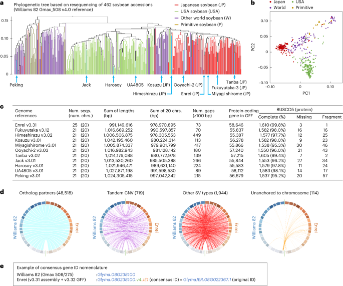
a, Phylogenetic tree of 462 worldwide soybean cultivars and varieties. The analysis was conducted using a resequencing (SNPs and short indels) dataset based on the Williams 82 Gmax_508 v4.0 reference. One wild soybean accession was used as an outgroup taxon. b, Principal component analysis of 462 soybeans based on the dataset used in a. c, Genome assembly and annotation statistics in newly constructed genomes. The ‘Num. gaps’ values indicate the number of gaps with ≥100 bp on 20 chromosomes. BUSCO5 benchmark²⁸ was used to evaluate the completeness of the protein sequence datasets. chrs., chromosomes; num., number; seqs., sequences. d, Circos plots comparing the Enrei and Williams 82 Gmax_508 genome references. One-to-one orthologous gene partners (48,518 links) are indicated by blue (genes are located in the same direction) and gray (genes are located in the opposite direction) lines. Purple, red and orange links indicate 719 tandem copy number variations (CNV), 1,944 other SV types and 114 genes that were unanchored to either genome, respectively. e, Gene ID nomenclature in the Enrei v3.31 genome reference. The consensus gene ID started with a ‘Glyma.’ string attached to Enrei genes that have one-to-one orthologs in either version of Williams 82 v4.0, v2.0 or v1.0 (see also Supplementary Fig. 5).

Full size image

Next, gene prediction was performed for the 11 genomes, mainly based on ONT RNA sequencing. We identified 55,387 to 58,646 protein-coding genes within them (Fig. 1c and Supplementary Fig. 4). The BUSCO5 benchmark²⁸ showed that the Enrei genome annotation (v3.32 General Feature Format (GFF)) represented the highly comprehensive dataset of plant protein-coding genes compared with the other soybean genomes (complete BUSCO, 99.8%; Fig. 1c). Then, the gene partner relationships between Enrei v3.31 and three versions of the Williams 82 reference genome (v4.0, v2.0 and v1.0) were investigated. The highest number of orthologs was observed when the Enrei and Williams 82 v4.0 genomes were compared (Fig. 1d), but the numbers differed slightly when other versions of Williams 82 were used for comparison (Supplementary Fig. 5a,b). As some genes, including PDH1 (Glyma16g25580), were absent from the Williams 82 v4.0 reference but present in the previous version (v1.0), we integrated the results of the three comparisons in a non-redundant manner (Supplementary Fig. 5c). As a result, of the 58,646 nuclear genes in the Enrei genome, 49,235 genes showed a one-to-one orthology relationship with the Williams 82 genes (Supplementary Data 2). We assigned a consensus gene ID to the orthologous genes of the Enrei genome (starting with the string ‘Glyma.’ and ending with ‘.JE1’) for consistency in gene nomenclature among soybean genomes (Fig. 1e).

Gene-SV and differentially expressed genes

In general, SVs can occur flexibly between individual genomes, and several patterns of gene disruption may be present per gene (Fig. 2a). Describing and analyzing SVs based solely on the conventional variant call format (VCF) is sometimes difficult. To explore the role of SVs, especially gene-SVs, in the diversification of global soybean genomes, we developed Asm2sv, a new assembly-based comparative genomics pipeline²⁴. This tool was designed to analyze gene-SVs in the context of flanking sequence alignments by calculating the degree of disruption of each gene as a numeric score (Fig. 2b and Supplementary Fig. 6). Asm2sv uses one genome reference as the base reference, and if a gene is disrupted by insertion or deletion in the target genome, the resultant gene-SV score for the gene shifts from 1.0 according to the degree of structural change. These gene-SV scores can be combined and used for subsequent analysis on a population scale. In addition to gene-SV score calculation, Asm2sv can also output VCF data based on the gene-level SV analysis, which can be used for pangenome construction (see later sections).

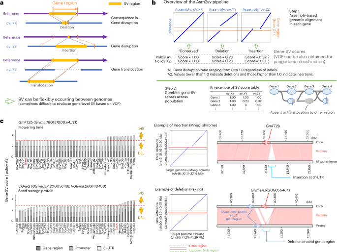
a, Schematic illustration of the flexible SV that may be detected between distinct genomes. b, Overview of the Asm2sv pipeline. This pipeline was designed to capture flexible SVs in each gene region based on algorithmic genomic alignment. The degree of gene conservation, disruption or extension in the target genome is calculated as a numeric score. The gene-SV scores can be combined to compare multiple genomes. Asm2sv can also output VCF data to use for pangenome construction. The detailed principles and usage of this pipeline are described in Supplementary Fig. 6. c, Examples of gene-SVs detected by Asm2sv. Gene-SV scores and genomic alignments are shown for the GmFT2b and CG-α-2 genes that carry insertion or deletion SVs, respectively. The left panels indicate bar charts showing the gene-SV scores obtained by Asm2sv; the center and right panels indicate examples of genomic alignment and microsynteny, respectively. In the left panel, the cultivar Enrei is highlighted in red text as its genome was used as the base reference.

Full size image

With the Enrei v3.31 genome used as a base reference, we applied the Asm2sv pipeline to the genome assemblies of 42 global soybean cultivars and varieties, 31 of which originated from previously reported data^9,14,18,19 (Supplementary Table 1). Figure 2c shows examples from the Asm2sv analysis. In particular, a 3.5 kb insertion was detected around the 3′ untranslated region (3′-UTR) of a flowering regulator gene, GmFT2b (Glyma.16G151000.v4.JE1), in Miyagi shirome and Tanba, while a disruptive deletion was detected around a seed storage protein gene, CG-α-2 (GlymaJER.20G056481.1/Glyma.20G148400), in ‘Jack’ and ‘Peking’. According to the genome-wide view of gene-SVs shown in Fig. 3a, most genes appeared to be conserved between the 42 genomes. However, there were some SV-prone regions such as the upper part of chromosome 3 (chr3) and the bottom part of chr16. Around these regions, the cumulative gene-SV scores exhibited significantly lower values than those of the other positions (Fig. 3a). When the threshold was set to 29 (conserved ratio of ≤70%), 1,518 genes and transposon elements were selected as the less-conserved group (Fig. 3a and Supplementary Data 3). One of the benefits of using Asm2sv’s gene-SV score data is that they can be directly applied to gene-level analyses, such as term enrichment analysis (TEA). Accordingly, TEA indicated that specific InterPro terms, such as IPR032675 (leucine-rich repeat domain superfamily), IPR044974 (plant disease resistance protein) and IPR002182 (NB-ARC), were overrepresented in the less-conserved group together with retrotransposon-related terms (Fig. 3b). This suggests that nucleotide-binding site leucine-rich repeat (NBS-LRR) genes could be variable compared to other genes between soybean genomes. When hierarchical clustering was performed based on the gene-SV score data, 42 soybean genomes were divided into three groups (Fig. 3c). Cultivated and wild soybeans were separated into different clades, and cultivated soybeans were further separated into two clades: G. max I and II. In particular, Japanese soybeans were clustered into the G. max I clade. This clade diverged from G. max II, consisting of Chinese and US germplasms, consistent with the phylogenetic trees presented in Fig. 1a. We also performed Asm2sv analysis using recently published telomere-to-telomere (T2T) gap-free genomes of Williams 82 and Jack^20,21 (Supplementary Fig. 7a,b). Gene-SV scores were almost identical between the T2T and non-T2T genomes, probably because gene-rich regions, which are the target of Asm2sv analysis, are sufficiently assembled even in non-T2T genomes. Accordingly, hierarchical clustering was not affected by the addition of T2T genomes (Supplementary Fig. 7b).

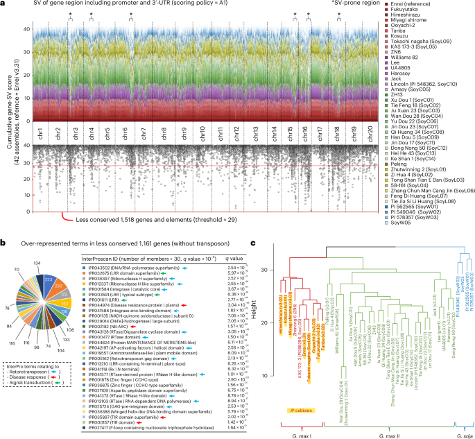
a, Cumulative gene-SV scores obtained by Asm2sv in 42 soybean genomes. The Enrei v3.31 genome was used as the base reference. In the cumulative bar chart shown in the top panel, soybean genomes are indicated by different colors. The dot plot in the bottom panel is presented to emphasize the genes or elements that are less conserved between these genomes (the red box). Some examples of SV-prone regions were marked by asterisks as they exhibited a sharp downward peaks. b, Overrepresented terms in the less-conserved genes and elements shown in a. TEA was performed based on the InterPro ID. The q values were calculated from P values obtained by two-tailed Fisher’s exact test. Terms relating to three different categories (retrotransposon, disease response and signal transduction) are indicated by light blue, red and green arrows, respectively. AP, apoptotic protease; RTase, reverse transcriptase; TIR, toll/interleukin-1 receptor. c, Hierarchical clustering of 42 soybean genomes based on gene-SV scores. Cultivated and wild soybeans are shown in different colors; Japanese soybeans are indicated by red characters with a yellow background.

Full size image

Then, we analyzed RNA-seq data from various tissues of Enrei and Williams 82 to gain insights into differentially expressed genes (DEGs) (Fig. 4a). When 44 transcriptomes were subjected to weighted genome-wide co-expression network analysis (WGCNA)²⁹, 125 co-expression groups were identified in the dataset (Fig. 4b and Supplementary Data 4). Of these, 295 genes from five groups exhibited predominantly upregulated gene expression in Enrei relative to Williams 82, whereas 216 genes from six groups were upregulated in Williams 82 (fold change of ≥2 and P value < 0.01; Fig. 4c,d). TEA indicated that defense response-related InterPro terms, such as IPR002182, IPR044974 and IPR032675, were again overrepresented in these DEGs, together with retrotransposon-related terms (Fig. 4e). When comparing 511 DEGs with the 1,518 less-conserved genes and elements described above, only 65 were found to overlap (Supplementary Data 5). This suggests that gene-SV does not necessarily activate or suppress gene expression in an all-or-nothing manner. Nevertheless, it is likely that disease response-related genes, together with retrotransposons, exhibit greater variability across soybean genomes than other genes.

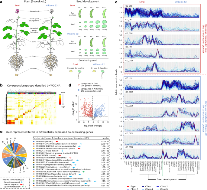
a, Schematic illustration of tissue-wide RNA-seq dataset for Enrei and Williams 82. b, Heatmap illustrating the co-expression groups identified by WGCNA²⁹. c DEG groups identified by comparison between Enrei and Williams 82. The red lines indicate the expression patterns of computationally calculated eigengenes that represent the co-expression group. Genes were categorized into a co-expression group according to P values that were calculated by WGCNA (P < 1 × 10⁻⁶, n = 44). d, Volcano plot showing the significance levels of each DEG. To identify genes predominantly expressed in either genotype, P values were calculated with two-tailed Student’s t-test based on the all-expression levels in 22 tissues of Enrei and Williams 82 (P value < 0.01 and fold change of ≥2). Genes belonging to the co-expression groups shown in c were analyzed. The red and blue dots indicate Enrei-upregulated or Williams 82-upregulated genes, respectively. e, Overrepresented terms in Enrei-upregulated or Williams 82-upregulated gene groups identified in d. TEA was performed based on the InterPro ID. The q values were calculated from P values obtained by two-tailed Fisher’s exact test. Terms relating to three different categories (retrotransposon, disease response and signal transduction) are indicated by light blue, red and green arrows, respectively.

Full size image

Genomic region that distinguishes Japanese soybeans

Next, we attempted to identify gene-SVs that distinguish members of the G. max I and II clades (Fig. 3c). Given that gene-SV data were obtained as numeric scores in Asm2sv, P values were calculated using the two-tailed t-test between the two groups. The resultant plot indicated the presence of several peaks across the genome, with the most prominent one observed around 29.91–32.58 Mb on chr16, where the PDH1 gene is located (Fig. 5a and Supplementary Data 6). However, because we could only use 42 genome assemblies, it was difficult to obtain a conclusive result. Thus, we used short-read datasets from 462 soybean lines to prepare a combined VCF dataset that included both SNPs and SVs. SNP and short insertion and deletion (indel) data, obtained through conventional resequencing analysis based on the Enrei genome, were integrated with SV data derived from pangenome analysis using resequencing datasets. For the latter, the pangenome reference was initially constructed using 12 soybean genomes, including 11 ONT-assembled genomes from this study and a previously published T2T genome of Williams 82 (ref. ²⁰). For this purpose, not only SVs inferred with published tools^30,31 (for example, Minigraph-Cactus) but also those obtained by Asm2sv were used as hints (see Methods for details). Our preliminary analysis indicated that insertion or deletion SV of GmFT2b and CG-α-2, which were detected by assembly-based comparison in Fig. 2c, could also be detected in the combined VCF data when Asm2sv’s SV data were used for pangenome construction (Supplementary Fig. 8). Given that published tools alone failed to detect these SVs, Asm2sv was deemed useful for SV detection. When a selective sweep scan was performed using the combined VCF data between 140 Japanese and 176 US soybeans, sharp peaks were observed in several genomic regions (Fig. 5b). Among them, peaks around 29.91–30.93 Mb on chr16, 11.47–12.40 Mb on chr17 and 45.51–46.32 on chr3 exhibited cross-population composite likelihood ratio (XP-CLR) scores³² above 1,500, and some of these were identical to those found in the score-based t-test analysis (compare Fig. 5a,b). We also tested other comparisons (for example, East Asian versus US soybeans), but the selective sweeps were much weaker than those of the Japanese–US comparison (Fig. 5b and Supplementary Fig. 9). These results again indicated that genome sequences were diversified, especially between Japanese and US soybeans. Interestingly, the PDH1 gene was found to be located within the Japanese–US selective sweep peak around the bottom of chr16. A previous study²⁵ genetically demonstrated that a loss-of-function pdh1 allele caused by a K31* stop-codon mutation results in enhanced pod-shattering resistance in soybean²⁵. Fig. 5c clearly indicates that almost all US soybean lines carried the pdh1 allele (K31* mutation), while most Japanese lines carried the wild-type PDH1 allele, suggesting that the PDH1 gene is a leading candidate for the Japanese–US selective sweep. Nearly half of the East Asian lines, except the Japanese ones, carried the pdh1 allele, suggesting that this allele initially originated in these accessions and then became predominant in US cultivars.

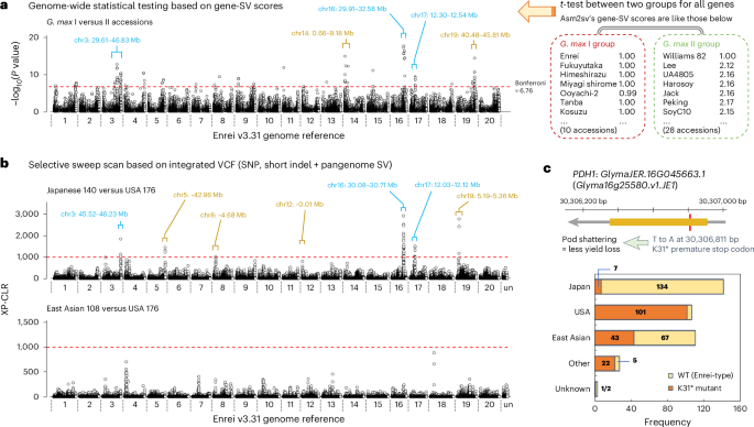
a, Manhattan plot of gene-SVs that distinguish G. max I and II members. Two-tailed Student’s t-test was performed based on gene-SV scores between 10 G. max I and 28 G. max II soybean lines, as described in the right panel. The Bonferroni-corrected threshold for P = 0.05 is indicated by a red dashed line. Positions of significant −log₁₀(P value) peaks are indicated by square braces, and lines which overlap with XP-CLR peaks in b are shown in light blue. b, Genome-wide selective sweep scan using XP-CLR³². The top panel indicates the comparison between 140 Japanese and 176 US soybeans; the bottom panel compares 108 East Asian (except Japanese) and 176 US soybeans. The XP-CLR values were calculated based on the VCF data that integrated conventional resequencing datasets (SNPs and short indels) and pangenome SV datasets. For clarity, primitive soybean accessions were not included in these analyses. Positions of significant XP-CLR peaks are indicated by square braces, and lines which overlap with gene-SV peaks in a are in light blue. c, The frequency of the stop-codon mutation (K31*) of the PDH1 gene in Japanese and other soybeans. Note that this mutation leads to increased pod-shattering resistance²⁵.

Full size image

GWAS on the seed size and shape of Japanese soybeans

Japanese soybeans produce relatively large and round seeds compared to others (Fig. 6a). To identify the genomic regions associated with these seed traits, GWAS were conducted using the phenotype and genotype datasets of 125 Japanese and 96 global soybeans (a total of 221 lines). For this purpose, we first measured the seed area size, length and width using SmartGrain software³³ (Fig. 6b and Supplementary Fig. 10). By analyzing seeds obtained from cultivations in three independent years (2021, 2022 and 2023), some Japanese soybeans were confirmed to exhibit larger seed sizes than others (Fig. 6c and Supplementary Data 7). Of these, the seeds of eight Japanese landraces, including Tanba, were especially big, probably associated with their specific and traditional food uses, such as boiled soybeans and edamame. Roundness was estimated by calculating the ratio of length to width, and the frequency of soybean lines with round seeds was also slightly higher in Japanese lines than in others. In both horizontal and vertical measurements, correlations were found between area size, length and width, indicating that these parameters represented seed size (Fig. 6d). By contrast, no correlation was observed between area size and roundness. We also quantified the oil and protein content in these seeds (Supplementary Fig. 10c and Supplementary Data 8). However, these levels did not differ between Japanese and other soybeans.

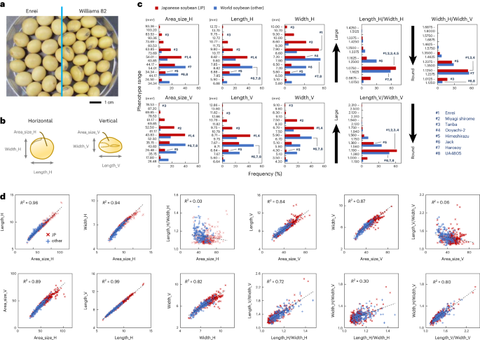
a, Photographs of the seeds of Enrei and Williams 82. b, Cartoon illustrating the definition of seed area size, length and width. These values were quantified with SmartGrain software³³, both horizontally and vertically. c, Histograms showing the frequencies of seed area size, length and width in Japanese and other world soybeans. The ratios of length to width or horizontal width to vertical width were calculated to represent seed roundness. Seeds were obtained from 221 soybean lines cultivated in 2021, 2022 and 2023 (n ≥ 536). The positions of soybean lines whose genome references were constructed in this study are shown by dark blue numbers. d, Dot plots showing correlations between seed phenotype parameters. The coefficients of determination described in the plots were calculated by linear regression (n = 520).

Full size image

In the GWAS, we focused on seed size and shape (roundness). Two variant datasets—one derived from conventional resequencing analysis (SNPs and small indels) and another from pangenome analysis (mainly SVs)—were separately used for GWAS to calculate P values. The quantile–quantile (Q–Q) plots showed that the population structure among the 221 soybean lines was effectively corrected by the mixed linear model and FarmCPU (Supplementary Figs. 11 and 12). By evaluating the SNP-based and SV-based GWAS together, we identified several candidate QTL peaks for eight seed-related phenotypes across the genome (Figs. 7a and 8a). Notably, of the 388 candidate variants associated with these phenotypes, 146 were identified through SV-based GWAS (Supplementary Data 9). Given that SV-based GWAS peaks overlapped with those from SNP-based GWAS (Figs. 7a and 8a), these variants were probably co-segregating within the soybean population. Interestingly, the positions of the two seed size-associated peaks were very close to or overlapped with selective sweeps (for example, ~31.66 Mb on chr16 and 10.45–13.21 Mb on chr17). Several prominent peaks were also observed in other genomic regions, despite not overlapping with selective sweeps. Detailed analysis of DNA variants within the 4.24–6.58 Mb region on chr7 (seed size 7-1) and the 10.45–13.21 Mb region on chr17 (seed size 17-1) revealed at least two independent variants within each region that additively influenced seed size (Fig. 7b,c). Notably, specific allele combinations within both QTL regions were found to significantly increase seed size, and these combinations were predominantly found in Japanese soybeans, whereas they were almost absent in other populations. When examining DNA variants near the bottom of chr16, seed sizes could be separated by the ~3 kb SV located at 31,677,586 bp, which was 1 Mb apart from PDH1 (Fig. 7d). This SV appeared to be a presence–absence variation of a retrotransposon located upstream of the putative GATA transcription factor gene (Glyma.16G152700.v4.JE1), whose gene expression is specific to developing seeds (Supplementary Fig. 13). The impact of this SV on seed size was independent of PDH1 and was observed exclusively in Japanese soybeans (Fig. 7d), suggesting that its function might be linked to some background factor(s). Additionally, Japanese soybean-specific SV alleles that increased seed size were identified at 742,232 bp on chr4 and 1,362,354 bp on chr18 (Fig. 7e,f). Notably, across all five QTLs shown in Fig. 7b–f, eight Japanese landraces with particularly large seeds carried the variant alleles and their combinations that contributed to increased seed size.

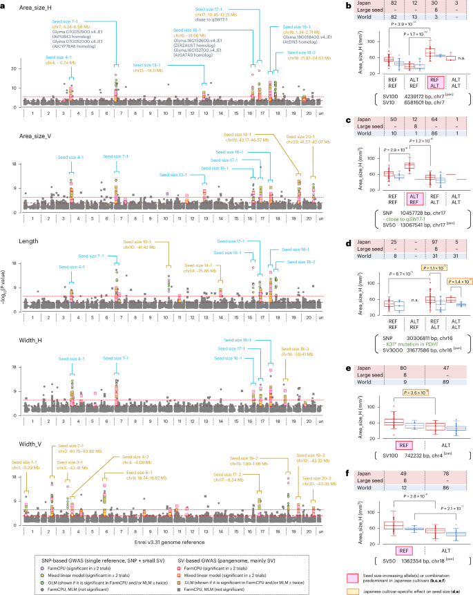
a, Manhattan plots showing the results of the GWAS. Seed area size, length and width in 221 soybean lines (Fig. 6) were used as the phenotype data. The −log₁₀(P values) were separately calculated using the rMVP tool⁴⁴ with the VCF data from single-reference (SNPs and short indels) or pangenome (SV datasets) analyses. The corrected significance thresholds that were calculated using rMVP in SNP-based or SV-based GWAS are indicated by red dotted and dashed lines, respectively, in the plots. For each phenotype, a plot was created by combining the results of independent GWAS that were conducted based on the phenotype data of three years (2021, 2022 and 2023) and their averages. In rMVP, the general linear model (GLM), mixed linear model (MLM) and FarmCPU were used, but the −log₁₀(P values) from the GLM are presented in the plots only when those of MLM and/or FarmCPU tests for the variant were above the threshold level in at least two tests. The positions of significant −log₁₀(P value) peaks are indicated by square braces and lines together with candidate gene IDs (if present). The −log₁₀(P value) peaks that were commonly observed between distinct phenotype parameters are highlighted in light blue. b–f, Box plots showing the effect of variants on seed size. The combined effects of two variants are analyzed in b–d. The frequencies of Japanese and other world soybeans are indicated separately by different colors. For box plots, the center line denotes the median value; the box contains the 25th to 75th percentiles of the dataset; whiskers extend 1.5 times the interquartile range; and dots represent individual phenotype values. P values calculated by two-tailed Student’s t-test indicate significant differences between groups. SV10, SV50, SV100 and SV3000 indicate 10–50 bp, 50–100 bp, 100–1,000 bp and 3–5 kb differences between reference and target genomes, respectively. REF and ALT indicate reference and non-reference genotypes, respectively. SVs obtained through pangenome analysis are indicated by ‘[pan]’. ‘Large seed’ indicates eight Japanese landraces with particularly large seeds that were selected by the following criteria: averaged area_size (H) > 80 mm² and averaged area_size (V) > 60 mm² (see also Supplementary Data 7).

Full size image

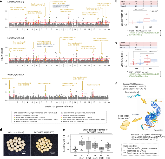
a, Manhattan plots showing the results of the GWAS. Ratios of length to width and horizontal width to vertical width in 221 soybean lines (Fig. 6) were used as seed shape (roundness) parameters. The −log₁₀(P values) were calculated by the same method described in Fig. 7. The positions of significant −log₁₀(P value) peaks are indicated by square braces and lines together with candidate gene IDs (if present). b,c, Box plots showing the effect of the candidate variant within Glyma.08G168400.v4.JE1 (b) and Glyma.09G048300.v4.JE1 (c), which are soybean homologs of the Arabidopsis genes EPIDERMAL PATTERNING FACTOR 2 (EPF2) and GSO1/SGN3, respectively. The frequencies of Japanese and other world soybeans are indicated separately by different colors. P values calculated by two-tailed Student’s t-test indicate significant differences between groups. ‘Large seed’ indicates eight Japanese landraces with particularly large seeds that were selected by the following criteria: averaged area_size (H) > 80 mm² and averaged area_size (V) > 60 mm² (see also Supplementary Data 7). d, Photographs of the seeds of induced soybean mutants. Unlike wild-type Enrei (WT), the EnT-6455 mutant carried the A560T amino acid substitution mutation within Glyma.09G048300.v4.JE1. e, A boxplot showing the frequencies of seed shape in the segregating progenies of the EnT-6455 mutant. Genotypes of each segregant are also shown in the plots; their parent is homozygous ALT (ALT), heterozygote (Htz) or no mutation (REF). The ratio of horizontal length to width was quantified in biologically independent individual seeds with SmartGrain software³³ (n = 30 for wild-type Enrei, n ≥ 15 for ALT and Htz genotypes, n = 10 for REF genotype). f, Cartoon illustrating a possible member of the seed-specific TWS1-GSO1/SGN3 signaling component in soybeans. Four genes are described as possible candidates that may have a role in the regulation of seed shape in soybeans. The 3D structure images of soybean GSO1/SGN3 and TSW1 homologs were obtained using the AlphaFold 3 (ref. ⁴⁵). SERK, SOMATIC EMBRYOGENESIS RECEPTOR-LIKE KINASE. For box plots in b, c and e, the center line denotes the median value; box contains the 25th to 75th percentiles of the dataset; whiskers extend 1.5 times the interquartile range; and dots represent individual phenotype values.

Full size image

In addition to seed size, candidate DNA variants were also found for seed shape. For instance, the SNPs positioned at 13,578,035 on chr8 and 4,173,587 bp on chr9 had relatively strong effects on seed shape in both Japanese and other soybeans (Fig. 8a–c). The SNP on chr8 was found within the intron of Glyma.08G168400.v4.JE1, a soybean homolog of the Arabidopsis EPIDERMAL PATTERNING FACTOR 2 (EPF2) peptide signal gene³⁴. The latter SNP caused L147F amino acid substitution mutation in Glyma.09G048300.v4.JE1, whose gene expression is specific to pods and developing seeds (Supplementary Fig. 14). Interestingly, this gene was a homolog of the Arabidopsis GSO1/SGN3 gene, an LRR receptor gene known to perceive the peptide signal TWISTED SEED 1 (TWS1)³⁵. Given that the TWS1-GSO1/SGN3 pathway is known to regulate seed shape in Arabiodopsis³⁵, we further screened the soybean-induced mutant library of the Enrei background³⁶. As a result, one mutant, designated EnT-6455, was found to carry an A560T amino acid substitution (Supplementary Figs. 15 and 16). This mutant also exhibited oval seed shape and wrinkled seed coat phenotypes compared to the wild type (Fig. 8d,e), which might be similar to Arabidopsis gso1 gso2 double mutants³⁷. According to the homolog search, two soybean homologs for TWS1 were found in the Enrei genome: Glyma.14G087800.v4.JE1 and Glyma.17G236500.v4.JE1 (Supplementary Fig. 17). Like Glyma.09G048300.v4.JE1, their gene expression was specific to developing seeds, suggesting the possible role of the TWS1-GSO1/SGN3 protein complex in the regulation of soybean seed shape (Fig. 8f). Taken together, these results indicate that several QTLs are associated with seed size and shape. In particular, genetic variants within the GWAS peaks of chr7, chr16 and chr17 appear to account for large seed sizes in some Japanese soybeans.

Despite advances in DNA sequencing technologies, characterizing SVs remains challenging. In this study, we attempted to overcome this difficulty using ONT long-read sequencing to assemble soybean genomes. This resulted in the construction of 11 reference genomes, enabling both high-resolution comparative genomic analysis and SV detection by pangenome analysis. We present comprehensive evidence that our newly developed Asm2sv pipeline is useful for these analyses. First, based on the assembly-based gene-SV analysis of 42 worldwide soybean genomes, gene-SV score data successfully reflected the genetic relationships between three distinct groups (Fig. 3c), with G. max clade I, including Japanese soybeans, clearly separated from G. max clade II. This was consistent with the phylogenetic tree analysis shown in Fig. 1a, demonstrating that Asm2sv’s gene-SV score data can be used to distinguish between genomes. One of the advantages of using such gene-SV score data is their direct applicability to TEA-like studies. Indeed, specific InterPro terms were found to be enriched in the less-conserved gene group among the 42 soybean genomes (Fig. 3b). Although retrotransposon-related terms were frequent in the less-conserved group, reflecting their role as mobile elements, most other enriched terms were related to the defense response. Notably, NBS-LRR genes (putative R genes) were exclusively abundant. In general, NBS-LRR genes comprise a tandem cluster in plant genomes³⁸. Hence, unequal crossing over, sequence exchange or gene conversion may lead to variations in these genes^39,40. Such variation in NBS-LRR genes may collectively contribute to defense response, including nonhost resistance^41,42 and interaction with other helpful microorganisms. In this context, it was also an interesting observation that NBS-LRR genes were overrepresented in DEGs between Enrei or Williams 82 (Fig. 4e). It is possible that they may have arisen as a consequence of breeding under different conditions (for example, climate and microbiome) between countries.

Another important feature of Asm2sv is that it can also produce VCF data based on gene-level SV analysis. Our results demonstrated that the Asm2sv-based pangenome reference could detect 3.5 kb or 6.7 kb SVs of GmFT2b and CG-α-2, respectively, which could not be achieved with published tools alone (Fig. 2c and Supplementary Fig. 8). In this study, this advantage contributed to the GWAS (Figs. 7a and 8a). Our SV-based GWAS successfully identified several candidate variants associated with seed size (Fig. 7a). Together with variants found through SNP-based GWAS, we identified several alleles that accounted for the large seed size of some Japanese soybeans (Fig. 7b–f). For example, eight Japanese landraces with particularly large seeds were found to carry allele combinations that increase seed size in all five major QTLs identified in the GWAS. Given that large-seed grains are essential for producing some traditional soy foods, it is possible that these variants, including SVs, have been key in breeding cultivars for these purposes. Of particular interest is the overlap between Japanese–US selective sweeps and seed size QTLs (Figs. 5b and 7a). Our GWAS identified a QTL around 10.45–13.21 Mb on chr17, where a selective sweep also occurred. This finding is consistent with the previous identification of qSW17-1, a seed size QTL, around this region using genetic populations derived from crosses between Japanese and US cultivars⁴³. However, our high-resolution GWAS, which included both SV and SNP datasets, implied the presence of at least two causal genes for this QTL, as two independent variants were found to additively affect seed size (Fig. 7c). Unlike chr17, the Japanese–US selective sweeps and seed size QTL appeared to be 1 Mb apart from each other, around the bottom region of chr16 (Figs. 5b and 7a). For the selective sweep around 30.08–30.71 Mb on chr16, the PDH1 gene emerged as the leading candidate gene responsible for pod-shattering resistance, as previously demonstrated genetically²⁵. Most Japanese soybeans carry the wild-type allele of PDH1, whereas the loss-of-function pdh1 allele is predominant in US cultivars (Fig. 5c). This is possibly related to circumstances specific to Japan. Owing to the limited availability of flat farmlands in Japan, large-scale agricultural mechanization was delayed during the 20^th century. This may have compelled farmers to maintain soybean cultivars with reduced pod-shattering resistance (wild-type PDH1 allele) because manual threshing would be difficult with hard-shattering pods. As mentioned above, Japanese landraces with particularly large seeds (for example, Tanba) carry the SV allele that increases seed size at the neighboring QTL (~31.66 Mb on chr16). As these soybeans are used for the production of traditional soy foods, the presence of this seed size QTL may be another reason for the preservation of the wild-type PDH1 allele in these cultivars.

Although phenotypic differences in seed shape between Japanese and other soybeans were less significant than those in seed size, seed shape remains an important trait for Japanese soybeans because both the local people and the food industry prefer round-shaped beans. Our GWAS identified a GSO1/SGN3 homolog, Glyma.09G048300.v4.JE1, as a candidate gene for this trait (Fig. 8a,b). In Arabidopsis, the GSO1/SGN3 receptor perceives the TWS1 peptide signal, which controls seed shape^35,37. Consistent with this concept, we proposed a similar role for the soybean GSO1/SGN3 homolog. First, the expression of Glyma.09G048300.v4.JE1 was specific to pods and developing seeds (Supplementary Fig. 14). Second, the induced mutant for this gene showed an oval seed shape, consistent with the GWAS showing that an amino acid substitution variant is associated with this phenotype (Fig. 8d,e). Although further genetic complementation testing is necessary to eliminate the possible effects of background mutations, our results collectively suggest that this gene is one of the factors responsible for seed shape variation in soybean.

In conclusion, our study presents a proof-of-concept for using Asm2sv to investigate gene-SVs. However, challenges may arise when applying this pipeline to pangenome studies. Although this method was effective in detecting simple indel SVs, such as those in CG-α-2 and GmFT2b, analyzing more complex SVs, like super tandem repeats spanning more than 1 Mb, may be difficult. To address these challenges, the use of ultra-long sequencing with reads exceeding 1 Mb and/or compiling multiple T2T genomes may be beneficial. Finally, we provide a web database, designated Daizu-net (https://daizu-net.dna.affrc.go.jp), as a platform to share tools and omics datasets for functional genomic studies of Japanese soybeans (Supplementary Fig. 18). In future studies, additional assemblies, resequencing data and transcriptome data will be made available in this database. Such efforts will further promote the identification of causal genes for the seed size and shape QTLs identified in this study as well as support the breeding and cultivation of soybean as a global food security crop.

Plant materials, growth conditions and phenotyping

G. max cultivars, varieties and other germplasms were obtained from the NARO GenBank in Japan. To prepare total RNA, plants were grown in a soil mixture composed of Nippi (Japan Agricultural Cooperatives) and SuperMix (Sakata Seed Corp.) (v/v: 2:1) at 28 °C under 16 h light, 8 h dark cycles in air-conditioned greenhouses. The soil was inoculated with Rhizobium and Azospirillum (Tokachi Nokyoren) to facilitate plant growth. Root nodule samples were independently prepared from plants cultivated in pots containing vermiculite GL (Nittai) and watered with a nitrogen-free plant nutrient solution 4 weeks after inoculation with Bradyrhizobium diazoefficiens USDA 110. The Bradyrhizobium strain was cultured for 5 days in yeast extract mannitol medium at 28 °C, and 10⁷ cells were inoculated into seeds in a vermiculite pot. To prepare genomic DNA, seedlings were grown at 27 °C under 12 h light, 12 h dark cycles in a growth chamber, and then hypocotyl and young leaves were harvested. For the isolation of genomic DNA or total RNA, harvested plant tissues were frozen in liquid nitrogen and stored at −30 °C or −80 °C, respectively.

To obtain phenotype datasets, seeds were obtained from cultivations in 2021, 2022 and 2023. Soybean plants were grown in the agricultural fields of the Institute of Crop Science, NARO, located in Tsukuba City, Japan. In brief, seeds were sown in three rows at a spacing of 10 cm between plants and 70 cm between rows. Nitrogen (N), phosphate (P₂O₅) and potassium (K₂O) fertilizers were applied at 30, 500 and 100 kg ha⁻¹, respectively, as basal fertilizer. For the NARO mini-core collection, at least 60 plants per genotype were grown; at least six plants per genotype were cultivated for others. Pods, including seeds, were harvested at the R8 (full maturity) stage, followed by hanging in the shed to dry naturally before threshing. To measure seed area size, length and width, photographs were taken in each accession using 30 seeds (both horizontally and vertically), followed by image analysis with SmartGrain³³ (Fig. 6b and Supplementary Data 7). Seed shape (roundness) was evaluated by calculating the ratio of length to width or that of horizontal width to vertical width. Soybean lines with particularly large seeds were selected based on the following criteria: averaged area_size (H) > 80 mm² and averaged area_size (V) > 60 mm². To determine the content of oil and protein, about 5 g of seeds from each accession were ground into a powder using a Retsch ZM 200 grinder (Retsch ZM 200, Retsch), followed by near-infrared spectroscopy (Inframatic 9500, PerkinElmer).

Genomic DNA isolation and short-read resequencing

Genomic DNA was isolated using a Maxwell 16 Tissue DNA Purification Kit (Promega) or NucleoBond HMW DNA kit (Macherey–Nagely). The isolated genomic DNA was treated with short-read Eliminator XS or XL kits (Circulomics). For ONT sequencing, a DNA library was prepared using a ligation sequencing kit, either SQK-LSK109 or SQK-LSK110 (Oxford Nanopore Technologies), according to the manufacturer’s protocol. DNA sequencing was performed using Nanopore Minion or Promethion devices coupled with flow cells. For the genome sequencing of Enrei, both R9.4.1 and R10.3 flow cells were used, whereas only R9.4.1 was used for sequencing others. Base calling was performed with ONT Guppy (v6.0 or higher). For Illumina 150 bp paired-end sequencing, we used the services of private analytics companies (Azenta Life Sciences and Novogene). We obtained short-read paired-end datasets of 392 soybean lines from a public database^{11,12,15,16,17}; those of 75 were newly obtained in this study (Supplementary Data 1). The latter dataset included five redundant data of the cultivar Enrei. These short-read data were subjected to Trimmomatic⁴⁶ to remove low-quality data before analysis.

RNA isolation and RNA-seq data acquisition

Total RNA was isolated using an RNeasy Plant Mini Kit (Qiagen) according to the manufacturer’s protocol. For ONT cDNA RNA-seq, poly-A mRNA was isolated using a NEBNext Poly(A) mRNA Magnetic Isolation Module (NEB), and ONT libraries were prepared using a PCR-cDNA Barcoding Kit (SQK-PCS109, ONT). Sequencing was performed using ONT Minion coupled to an R9.4.1 flow cell. Base calling was performed using ONT Guppy (v6.0 or higher). For Illumina 150 bp paired-end RNA-seq, we used the service of a private analytics company (Eurofins Genomics).

Whole-genome assembly

In total, 11 G. max accessions were newly assembled in this study. The procedures, datasets, data amounts and detailed parameters used for the whole-genome assembly are summarized in Supplementary Fig. 1. For all accessions, contigs were first assembled using Canu (v2.2)⁴⁷ and/or NECAT⁴⁸. We used 158.9 Gb of ONT data for the Enrei genome, and the other genomes were assembled using 38.2–105.3 Gb of ONT data. Sequence errors within the contigs were corrected with Racon⁴⁹ and Medaka (https://github.com/nanoporetech/medaka) using ONT-read data. To identify candidates of chimeric contigs, ONT reads were again aligned to the contig sequences with Minimap2 (ref. ⁵⁰) using the following parameter: ‘-a -uf -k15 -A 2 -B 4 -O 4,24 -E 2,1’, followed by read-depth analysis using the mpileup function of samtools⁵¹. Contigs were split at positions where the depth of the ONT reads was <4. Errors that were still present in the contig sequences were further corrected three times with Pion⁵² using the Illumina paired-end dataset. For Enrei, scaffolds were assembled from contigs by combining a Bionano Saphyr optical map and Proximo Hi-C, which were obtained through the services of private analytics companies (AS ONE Corporation and Filgen). For Bionano scaffolding, 697 Gb of raw data was first assembled to construct a ‘cmap’ with Bionano Solve (v3.6.1); then, the cmap was used for scaffolding using the same pipeline. The Bionano scaffolds were further subjected to Juicer (v1.6) and 3D-DNA⁵³ coupled with Hi-C read data, followed by pseudomolecule construction based on previously reported genetic map information²⁷. Finally, the gaps were filled with contig datasets assembled under different conditions. For Fukuyutaka and ‘UA4805’, Bionano scaffolds were obtained by combining the contig assembly with 863 Gb or 942 Gb of raw Bionano data, respectively; then, a chromosome-scale pseudomolecule was constructed using a reference-guided strategy with Ragtag⁵⁴ and the Enrei genome. Pseudomolecule assemblies of other soybean lines were constructed directly from contigs using the reference-guided strategy. Finally, the JBrowse2 web application was set up on Daizu-net (https://daizu-net.dna.affrc.go.jp) according to the procedure described in a previous publication⁵⁵.

Gene prediction and identification of repetitive elements

Genome annotation was performed for all genomes assembled in this study. The procedures, datasets, data amounts and detailed parameters are summarized in Supplementary Fig. 4. First, by coupling datasets of 10.1 Gb ONT cDNA RNA-seq obtained from various tissues of the Enrei plant with the ONT4genepredict pipeline⁵⁶, 52,489 protein-coding genes were predicted. As complementary methods, gene prediction was performed using AUGUSTUS (v3.3.2)⁵⁷, Braker (v2)⁵⁸ or (v3)⁵⁹ and Genome Threader⁶⁰. For AUGUSTUS, the parameter dataset was first trained using an ONT-based annotation dataset, then gene prediction was performed. For the Enrei genome, Braker2 was executed using the Illumina RNA-seq dataset of tissue-wide samples (Fig. 4a); Braker3 was used for other genomes. Transcript annotation (information on the exon/intron structure) was performed using StringTie⁶¹ based on the same RNA-seq read alignment information. Genome Threader was executed based on the protein sequences of six published plant genomes: Arabidopsis thaliana (Araport13)⁶², G. max Williams 82 (v4.0, v2.0, v1.0)^3,9, P. vulgaris (v2.0)⁵, V. angularis (v1)⁶, Medicago truncatula (Mt4.0_v1)⁶³ and Lotus japonicus (v3.0)⁶⁴. EVidenceModeler (https://evidencemodeler.github.io) was used to integrate the results of StringTie, AUGUSTUS, Braker2 (or v3) and Genome Threader with weight scores of 10, 8, 1 and 1, respectively, producing a dataset of protein-coding genes. Finally, using the EVidenceModeler-based dataset as a supplementary dataset, the ONT-based annotation dataset was updated. The number of protein-coding genes in each genome is described in Fig. 1c. The BUSCO5 benchmark²⁸ coupled with the embryophyta_odb10 dataset was used to estimate the completeness of the protein sequence dataset. Finally, InterProScan5 (ref. ⁶⁵) was used to obtain the Gene Ontology and InterProScan ID for each predicted protein amino acid sequence. In addition, repetitive elements, including DNA and RNA transposable elements, were searched in the Enrei genome sequence using RepeatModeler2 (ref. ⁶⁶) and RepeatMasker (http://www.repeatmasker.org) with the library dataset dc20181026 (Supplementary Data 11).

One-to-one comparison of distinct genome references

Genome alignment was performed between distinct genome assemblies using LAST⁶⁷ with the following parameters: ‘-e 25 -v -q 3 -j 4 -P 32 -a 1 -b 1’ (for lastal) and ‘-s 35 -v’ (for last-split). After file format conversion by maf-convert, plot graphs comparing distinct genomes were generated using R (v3.6.3)⁶⁸ based on the LAST alignment results. A one-to-one comparison of two distinct genome references (for example, Enrei versus Williams 82) was performed as previously reported⁵⁶. In brief, to obtain information on orthologous partners, we performed bidirectional BLAST⁶⁹ searches using both transcript and protein sequences. We also used BLAT⁷⁰ to obtain supporting transcript alignment information. Genes from different genome references were considered one-to-one orthologous partners when they were paired in terms of a bidirectional BLASTN/P search, genomic positions, transcription orientation and exon/intron structures. Candidates for tandem copy number variation and other SV types (for example, translocating genes and presence–absence variations) were also identified as byproducts using these criteria. The one-to-one comparison analysis described above was automated in the Asm2sv pipeline²⁴. Circos software⁷¹ was used to visualize the results (Fig. 1d and Supplementary Fig. 5a,b). Consensus gene IDs were attached to genes of the Enrei reference genome by comparing them with three versions of Williams 82 references (v1.0, v2.0 and v4.0).

Gene-SV analysis based on the Asm2sv pipeline

The Asm2sv pipeline was developed based on a prototype script⁵⁶. This pipeline selects one genome reference as a base and analyzes gene-SVs based on algorithmic alignment analysis, as summarized in Supplementary Fig. 6. In this pipeline, a genomic sequence containing a query gene and its flanking region (x = 20 or 5 kb) was first obtained from the base genome sequence. Using this sequence as the query, a BLASTN search was performed against the target genome sequence. The specific region of the contig or chromosome that showed the best homology to the query sequence was selected from the BLAST search results. After masking the DNA sequence regions, except for the hit region, LAST was performed to obtain more detailed alignment data. If a candidate genomic region was identified in the target genome, changes in the genome structure (for example, deletion, insertion or extension) were analyzed at base-pair resolution for the gene, promoter and UTR based on the LAST alignment data. The length of the promoter and UTR was set to 5 kb in this study. Optionally, Asm2sv also attempts to identify open reading frames in the target genome based on protein alignment with Miniprot⁷² and Genome threader⁶⁰. If no candidate region was identified because of structural complexity, including the flanking region, alignment analysis was repeated using a reduced x value. Finally, the gene-SV score was calculated to determine the degree of gene conservation or disruption. We used two types of gene-SV scores, as shown in Supplementary Fig. 6: A1, which represents the gene disruption ratio, ranging from 0 to 1.0 regardless of indels; and A2, whereby values lower than 1.0 indicate deletions and those higher than 1.0 indicate insertions. For A1, scores close to 1.0 indicate that the genomic sequence and gene function are conserved between the base and target genomes, whereas scores close to 0 indicate that they collapsed owing to insertion or deletion in the target genome. In both cases, the score tables of multiple target genomes were combined to compare genotypes on a population scale. In this study, A1 data were used to identify less-conserved genes (Fig. 3a), whereas A2 data were used for cluster analysis to estimate the genetic relationships between accessions (Fig. 3c). The gene-SV data produced by Asm2sv were further used to identify those distinguishing the G. max I and II soybean cultivars (Fig. 5a). For this purpose, we performed two-tailed Student’s t-tests based on the numeric scores of the two groups to produce P values, which were used to generate a Manhattan plot. In addition to gene-SV score data, Asm2sv can output VCF data when ‘–vcf’ is specified in a command line. In this case, VCF data for each gene region was obtained based on the results of gene-SV analysis through read alignment using Minimap2 (ref. ⁵⁰) and SV calling with Sniffles2 (ref. ⁷³). VCF data derived from multiple genome assemblies were further combined with those of Minigraph-Cactus³¹ to construct a pangenome reference (see below).

Pangenome analysis based on multiple genome assemblies

To construct the pangenome reference, SV data were first obtained as VCF files using Minigraph-Cactus³¹. These data were based on 12 soybean genomes, which included 11 genomes assembled in this study (including the Enrei genome) and one previously published T2T genome of Williams 82 (ref. ²⁰). In parallel, additional VCF datasets were independently generated using Asm2sv. By using a custom script of Asm2sv²⁴, the VCF datasets from Minigraph-Cactus and Asm2sv were then integrated in a non-redundant manner, prioritizing Asm2sv’s SV data in cases for which overlaps occurred between the two methods. At this stage, multiple SV alleles from Asm2sv analyses were consolidated into a single representative SV, through multiple alignment with CLUSTALW⁷⁴, allowing genotype SVs to be treated as biallelic variants in certain cases (Supplementary Fig. 6). The resulting VCF data were used to construct a pangenome reference with Vg³⁰, using the Enrei genome as the base reference. Then, short-read data were aligned to the pangenome using Vg giraffe⁷⁵ with the parameters ‘–mismatch 1–gap-open 1–gap-extend 1–full-l-bonus 5’, followed by alignment data filtering using Vg filter with the parameters ‘-r 0.90 -fu -m 0 -q 5 -D 999’. After data processing with Vg pack, variant calling was performed using Vg call⁷⁶ with default parameters. The resulting genotype data contained numerous SVs larger than 1 kb in addition to small SVs (Supplementary Table 2).

Resequencing analysis based on a single-genome reference

Conventional resequencing analysis using either the Enrei or Williams 82 reference was conducted, as previously reported⁵⁶. In brief, short-read paired-end datasets were aligned to genome references with Bowtie2 (ref. ⁷⁷) using the following parameters: ‘–end-to-end–very-sensitive–score-min L,0,-0.12–mp 2,2–np 1–rdg 1,1–rfg 1,1’. After removal of secondary alignment and PCR duplicates with Samtools and Picard, respectively, variant calls were made using the Genome Analysis Tool Kit (v4.0)⁷⁸, and the effect of each DNA variant on the protein amino acid sequence was analyzed, as previously reported⁵⁶. According to the resequencing statistics, genotyping ratios were improved in the Enrei reference compared with those in Williams 82 when datasets were limited to Japanese soybeans (Supplementary Table 3). We confirmed that the phylogenetic tree of 462 soybeans based on the Enrei v3.31 genome was almost identical to that of the Williams 82 reference (Fig. 1a and Supplementary Fig. 19).

Phylogenetic tree analysis and PCA

For phylogenetic tree analysis and PCA, we used VCF data obtained through conventional resequencing methods. SNPs were first pruned using PLINK2 (ref. ⁷⁹) with the option ‘–indep-pairwise 50 5 0.5’, followed by PCA using the function ‘–pca var-wts’ in the same software. The dissimilarity matrix between soybean accessions was calculated with R-poppr⁸⁰ and then used to construct a phylogenetic tree using the neighbor-joining method implemented in MEGA (v11)⁸¹. The wild soybean accession ‘B01167’ was included as an outgroup.

Selective sweep analysis and GWAS

For selective sweep scanning, we used VCF data that integrated two variant datasets: SNP and short indel datasets obtained through conventional resequencing analysis based on a single-genome reference were combined with SV datasets obtained through pangenome analysis using resequencing datasets. An XP-CLR test³² was used to detect selective signatures between soybean accessions (https://github.com/hardingnj/xpclr). The XP-CLR value was computed using the following parameters: ‘–size 50000–step 10000–maxsnps 200’.

For GWAS, the SNP and SV datasets were separately used to calculate P values. In both datasets, DNA variants with a minor allele frequency of <0.05 were first removed, followed by genotype imputation with Beagle⁸² (v01Mar24.d36). Then, GWAS were conducted with the rMVP package⁴⁴ by setting the effective number of DNA variants estimated with gec.jar (https://pmglab.top/gec). For each phenotype, four independent GWAS were conducted based on the phenotype data of the years 2021, 2022 and 2023, as well as their averages. Although the general linear model, mixed linear model and FarmCPU were implemented in rMVP, the −log₁₀(P values) from the general linear model are shown in the Manhattan plot only when those of the mixed linear model and/or FarmCPU for the variant exceeded the threshold level at least twice in the four tests. For each phenotype, the −log₁₀(P values) from 24 tests (four phenotype samplings × three calculation methods × two genotype datasets) were combined to create a single Manhattan plot. For the Q–Q plot, the expected P values were calculated using R (v3.6.3) with the qqnorm function based on the observed P values.

TEA based on GO and InterProScan ID

TEA was performed based on a two-tailed Fisher’s exact test using R (v3.6.3) and the exact2x2 package. The R qvalue package was used to calculate the q value from the P value. This TEA is also available in the ‘GO enrichment analysis tool’ of Daizu-net (https://daizu-net.dna.affrc.go.jp/ap/got).

Transcriptome and co-expression analyses

Illumina RNA-seq paired-end short reads were subjected to Trimmomatic to remove low-quality data. Alignment was then performed with HISAT2 (ref. ⁸³) using the following parameters: ‘-k 1–maxins 1000–score-min L,0,-0.12–mp 2,2–np 1–rdg 1,1–rfg 1,1’. Gene expression levels were calculated as transcripts per million (TPM) values using StringTie⁶¹. After selecting genes with TPM ≥ 0.2 in at least nine samples (these are the expressing genes), WGCNA²⁹ was performed to obtain the co-expression dataset, as previously reported⁵⁶. The power thresholds were set to 12 for all analyses. In the WGCNA, the artificial numeric (eigengene) vectors representing the expression patterns of each co-expression group (module) were automatically calculated together with P values indicating the probability of module membership for each gene. We further calculated Pearson’s correlation coefficients using R (v3.6.3) between the TPM values of each gene and the eigengene vectors. Genes were categorized into co-expression groups when the P value was <1 × 10⁻⁶. Genes that were predominantly expressed in either Enrei or Williams 82 were identified by comparing the gene expression levels averaged across the tissue types; P values were calculated using two-tailed Student’s t-test and DEGs were identified by the following criteria: P < 0.01 and fold change ≥ 2.

Mutant screening and genotyping

The EnT-6455 mutant carrying the A520T amino acid substitution mutation in Glyma.09G048300.v4.JE1 (a soybean GSO1/SGN3 homolog) was obtained using high-resolution melting screening from the ethyl methanesulfonate-induced mutant library of the Enrei background, as reported previously³⁶. Primers used for high-resolution melting and genotyping are listed in Supplementary Data 12. For genotyping, dideoxy DNA sequencing was performed after PCR amplification⁸⁴. Eight seeds (siblings) were analyzed in each segregating progeny of the EnT-6455 mutant (Fig. 8d).

Statistics and reproducibility

All statistical tests were performed using the software, packages and online tools described in Methods. Our analyses are wholly reproducible using raw sequencing data from public databases and the command lines provided in the relevant Methods subsections (we used publicly available software for most analyses). GWAS were performed in 221 soybean lines using the seed size and shape phenotype datasets obtained over three years (2021, 2022 and 2023). Fisher’s exact test was used to assess the level of enrichment for InterPro terms, with statistical significance indicated by the q value. The sample size for tissue-wide co-expression analysis was determined based on previous studies. Co-expression was evaluated based on weight values calculated using R-WGCNA and Pearson’s correlation coefficients (n = 44).

Reporting summary

Further information on research design is available in the Nature Portfolio Reporting Summary linked to this article.