The interplay between the martensitic transformation rate and the rate of plastic relaxation during martensitic transformation in low-carbon steel, a phase-field study

Introduction
Low alloyed steels are among the most used materials for engineering applications due to their unique combination of properties, such as high strength and high toughness1,2. Steels with low content of alloying elements (usually less than 5% by weight), exhibit a desirable balance between cost, processability, and performance3. The composition of low alloyed steels typically includes manganese, silicon, chromium, molybdenum, and 0.05–0.25% wt.% carbon which contributes to the specific low alloyed steel characteristics4. Numerous industries, including automotive, construction, and aerospace, utilize low alloyed steels for their critical components. In automotive applications, for instance, these steels are utilized for their high strength-to-weight ratio, contributing to fuel efficiency and vehicle safety. In construction, the combination of strength and toughness makes low alloyed steels an ideal choice for structural components, such as beams and columns, capable of withstanding large loads and dynamic forces. Other industries, like shipbuilding and energy production, also benefit from these materials’ versatile properties5,6,7,8.
The properties of martensitic steels are determined by their microstructure, which is a result of the alloy composition and processing conditions9. To achieve the desired properties, it is crucial to understand and control the microstructural features, including grain size, precipitation, and phase distribution in the material10. The martensite transformation plays a crucial role in determining the final properties of low alloyed steels, with its effect on strength, ductility, and toughness11. Martensite transformation is a diffusionless solid-state phase transformation that occurs when the steel is cooled rapidly from the austenite phase, causing a change in the crystal structure from face-centered cubic (FCC) to body-centered cubic (BCC) for low carbon steels or to body-centered-tetragonal (BCT) for higher carbon content11. This transformation involves a shear distortion of the parent austenite phase, leading to the formation of martensite plates or laths with a specific crystallographic relationship12.
The thermodynamics and kinetics of martensite formation are governed by several factors, such as holding temperature, heat extraction rate, and chemical composition of steel13. The martensite start (Ms) and martensite finish (Mf) temperatures determine the range within which the transformation occurs, and these temperatures are influenced by the alloying elements present in steel14. The kinetics of martensite formation is also affected by the heat extraction rate, with faster rates leading to a more rapid transformation15.
The formation of martensite microstructures results in an increase in strength due to its fine microstructure and the trapping of carbon atoms within the BCT lattice16. However, this often leads to a reduction in ductility, as the martensite phase tends to display higher dislocation density and increased brittleness10. Therefore, understanding and controlling the martensite transformation kinetics is essential for optimizing the mechanical properties of low alloyed steels for specific applications.
A key aspect of martensite transformation kinetics is the interplay between the rapid martensitic transformation, which occurs at velocities comparable to the speed of sound in steel, and the process of plastic accommodation within the austenitic matrix. Here, the plastic deformation rate is a crucial factor in the martensite formation process, as it governs the mechanical behavior of steel during transformation-induced deformation17. High plastic deformation rates facilitate martensite nucleation and growth through two main mechanisms. First, they allow for rapid accommodation of the large transformation-induced strains, reducing the build-up of internal stresses that would otherwise oppose the transformation. Second, the increased dislocation density resulting from rapid plastic deformation can create additional nucleation sites for martensite, further promoting the transformation. This interplay between plastic deformation and martensitic transformation is crucial for understanding the kinetics and morphology of the resulting martensite structures. Conversely, lower plastic deformation rates can hinder the formation of martensite by increasing the nucleation barrier and decreasing the likelihood of local stress concentrations required for nucleation18.
Numerous studies have investigated the impact of prior plastic deformation on martensite formation kinetics, both through experimental and numerical means. Research has shown that martensite formation is facilitated when subjected to applied stress at higher temperatures, while pre-straining of austenite hinders the transformation19. Studies on 304 austenitic stainless steel grade reveal that strain rates affect martensitic transformation kinetics by interacting with environmental temperature, deformation heating, and strain rate sensitivity, ultimately influencing material strength and ductility18. A direct negative effect of strain rate on the martensitic transformation rate was found, which cannot be explained solely by adiabatic heating effects17. It was also observed that the strain hardening rate showed a strong connection to the current strain rate rather than the prior strain rate history17. It has been noted that the amount of plastic pre-straining does not significantly impact the kinetics of martensitic transformation, though it does affect the stress level required for initiating this transformation20.
In this study, a combined framework of phase field and phenomenological crystal plasticity is used to investigate the effect of plastic deformation during martensite formation. This approach builds upon significant advancements in the field, including the development of finite strain phase-field theories for martensitic transformations21,22 and the coupling of phase transformations with plasticity23,24,25,26. The phenomenological crystal plasticity models offer a powerful and robust framework for capturing the intricate deformation behavior of crystalline materials. While they do not explicitly track dislocation densities, the proper choice of empirical hardening law and carefully calibrated parameters enable an accurate representation of the macroscopic stress-strain response, as highlighted by27,28,29. One of the key strengths of the phenomenological approach lies in its computational efficiency. By avoiding the complexities of explicitly evolving dislocation densities, the model can be implemented in a computationally efficient manner, making it suitable for large-scale simulations and industrial applications30. Additionally, the model’s flexibility allows for the incorporation of various hardening laws and latent hardening effects, enabling it to capture a wide range of material behaviors.
The phase-field method has emerged as a powerful computational tool for studying various microstructural phenomena in materials science, including martensite transformation31,32,33. This method offers a mesoscale approach that enables the examination of intricate phenomena occurring at the interface between the atomic and macroscopic scales34, making it an effective way to model complex microstructural evolution35,36,37,38,39,40. The use of diffuse interfaces in the phase-field method greatly simplifies the numerical implementation by avoiding explicit tracking of interfaces41,42.
Recent phase-field studies of martensite formation have addressed various aspects of the transformation, such as martensite nucleation, growth, and variant selection43,44,45,46,47,48,49,50. These studies have provided valuable insights into the complex microstructural changes and interactions during the martensite formation process. In47, a phase-field model was presented to simulate martensitic transformation in steel, incorporating all 24 variants based on the Kurdjumov-Sachs orientation relationship (OR) and accounting for elastic strain effects during transformation, while using the Neuber elasto-plastic approximation to account for plastic deformation. Another phase-field model was developed to simulate martensitic transformation in steel, incorporating all 24 variants based on the Kurdjumov-Sachs OR and accounting for both elastic and plastic strain effects during transformation in small strain framework51. It was found that plasticity assists initial martensite nucleation but resists further growth in temperature-induced transformations, while transformation plasticity generates significant deformation even at stresses below the yield point in stress-induced transformations51. The interaction between phase transformations and plasticity has been a subject of intense research in recent years. Significant contributions include the development of phase field models for displacive phase transformations with plastic deformation52, the study of nanoscale mechanisms in mechanochemistry53, and the investigation of elastoplastic effects in martensitic transformations54. These works have advanced our understanding of the complex interplay between microstructural evolution and mechanical behavior in materials undergoing phase transformations.
However, challenges remain in developing phase-field models for martensite transformation, such as the need for accurate constitutive relationships, the calibration of model parameters55,56,57, and the high computational cost, especially for large-scale, three-dimensional simulations of full-complexity technical alloys47. Recent advancements in machine learning techniques have shown promising results in addressing some of these challenges, as highlighted in58, although these techniques are not employed in the present study.
Building upon the existing body of literature, our study investigates the interplay between the martensitic transformation rate and the rate of plastic relaxation in low alloyed steels. By systematically varying the plastic slip rate and heat extraction rate in phase-field simulations, we aim to elucidate how the material’s internal plastic response competes with the rate of the martensitic transformation. The simulations employ a newly developed finite strain elasticity solver59 integrated into the phase-field method to accurately capture the large deformations and local lattice rotations associated with the austenite to martensite transformation. Furthermore, the role of carbon content in influencing the transformation kinetics is explored. The resulting martensite microstructures, volume fraction evolution, internal stress development, and dilatometry curves are analyzed to provide insights into the complex kinetics of martensitic transformation in low alloyed steels. The findings of this study contribute to a deeper understanding of the interplay between the rapid martensitic transformation and the slower plastic accommodation, which is fundamental to understanding the resultant microstructure and its mechanical properties.
Results
The results presented in this section are based on comprehensive phase-field simulations of martensitic transformation in low-carbon steels. Before presenting our findings, we provide a brief overview of our simulation setup and methodology. For a complete and detailed description of the model formulation, computational methods, and parameters, readers are directed to the “Methods”.
The simulations described herein were conducted using the OpenPhase software library60, which implements a multi-phase field model coupled with crystal plasticity. The 3D computational domain was set to 12.8 × 12.8 × 12.8 μm3, discretized using 128 × 128 × 128 grid cells with the grid spacing of Δx = 0.1 μm. This grid size effectively balances the detailed representation of microstructural features with computational efficiency, as validated in47 and further confirmed in the present study. The phase-field evolution is simulated in the reference configuration with periodic boundary conditions. The micro-mechanical problem is solved using the fast Fourier transformation method to solve the mechanical equilibrium equation59 and phenomenological crystal plasticity30 to account for the plastic relaxation. The starting temperature for the simulations has been set to 673 °C, where austenite is the only stable phase for all steel grades considered in this study. All simulations were performed on a single crystal of austenite, allowing us to study the behavior of martensitic transformation without the influence of grain boundaries. The initial orientation of the austenite crystal was set to [100] along the x-axis, [010] along the y-axis, and [001] along the z-axis. Periodic boundary conditions were applied in all directions. The term ’variants’ is used throughout the manuscript to refer to the different K-S martensite variants that form within the single austenite crystal. The simulations focus on the martensite formation in steels containing 2 wt.% manganese, 1 wt.% chromium, and carbon contents varying between 0.1, 0.2, and 0.3 wt.%. The choice of steel grades is based on the parameters availability in prior investigation47. Martensite nucleation was simulated using a stochastic method. Nucleation sites were randomly distributed throughout the austenite matrix, with a density of ~1.0 × 10¹⁸ m−3 limited by the simulation resolution. At each nucleation site two martensite variants were randomly selected from the 24 possible Kurdjumov-Sachs variants. The critical nucleus size was set to 50nm in diameter, based on the assumption of preexisting martensite embryos reported in literature61. Note also, that all simulations in this study are using exactly the same pseudo-random sequence of generated nucleation sites and martensite variant pairs to avoid simulations inconsistency. Table 1 summarizes the key numerical parameters used in our simulations.
Time scale analysis of martensitic transformation
The kinetics of martensitic transformation is controlled by several interrelated factors: the rate of heat extraction responsible for the rise of thermodynamic driving force for the transformation; the rate of deformation propagation responsible for the lattice symmetry change between the austenite and martensite leading to the rise of the elastic energy which hinders the martensitic transformation; the rate of plastic accommodation of the transformation-induced deformation which reduces the elastic energy rise and facilitates further growth of the martensite. The kinetic coefficients Mαβ in Eq. (5) represent the numerical interface mobility which directly influences the transformation rate in the simulations. In our simulations, we have carefully adjusted the interface mobility along with other numerical simulation parameters, such as time step and plastic slip rate, to maintain simulations consistency across different cooling rates.
The simulation set described below was designed to investigate the interdependence between the rate of heat extraction, the rate of plastic deformation and the rate of martensitic transformation in low-carbon steel. Before the simulations could be performed a careful analysis of the time scales involved in the martensite formation has to be made based on the physics of the martensitic transformation.
It is well known that locally (at the atomic time and space scale) martensite formation occurs at velocities comparable to the speed of sound in steel. Considering the speed of sound in steel is ~5000 m/s62 and the typical interatomic spacing is around 1.5 Å, we can estimate the local transformation rate to be of the order of 1013 s−1 based on the time it takes for the transformation to propagate by a single interatomic distance. This represents the rate at which the transformation front propagates through the crystal lattice, causing the characteristic lattice deformation. However, globally (on the mesoscopic scale of microstructure) the volume fraction of martensite follows the rate of heat extraction which is a significantly slower process, e.g., with the rate around 1 s−1 for the effective cooling rate of 100 K/s. The plastic accommodation of the transformation-induced deformation occurs on the time scale close to the martensite formation rate on the atomic scale, e.g., close to the speed of sound in steel with the shear rate in the range of 1012 s−1 induced by the 20% characteristic transformation-induced deformation of martensite. On the other hand, the averaged transformation-induced shear rate on the mesoscopic scale, which follows the heat extraction rate, is of the order 10−1 s−1. Considering the difference in time scales involved in the martensitic transformation which is around 13 orders of magnitude, it is technically impossible to simulate the martensitic transformation on the mesoscopic scale following the speed of sound kinetics and at the same time covering the time range needed for the entire cooling process from the high temperature austenite state down to the complete martensitic state. Thus, in order to perform the microstructure formation simulations on the mesoscopic scale using the phase-field method we followed the martensite formation kinetics on the mesoscopic scale of microstructure and scaled the rate of plastic relaxation according to the transformation kinetics controlled by the heat extraction rate.
Effect of plastic slip rate on martensitic transformation
In the following, in order to observe the effect of plastic accommodation rate on the nucleation and growth kinetics of martensite, a set of simulations has been performed by varying the plastic slip rate across several orders of magnitude, from 1 × 10⁻² s−1 to 1 × 10⁻⁶ s−1. Here, a rate sensitive phenomenological crystal plasticity model formulation presented in “Methods” has been used. The effective cooling rate in these simulations has been set to 100 K/s and the steel grade with carbon content of 0.1 wt.% has been used. The simulations were performed down to room temperature and continued until the microstructure stopped evolving.
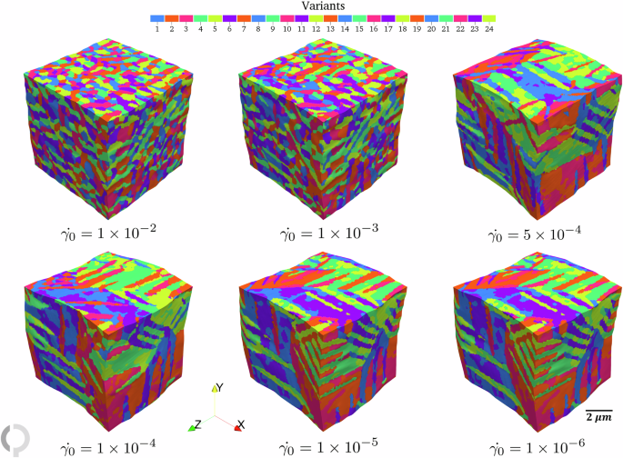
Figure 1 shows the volume fraction evolution for different plastic slip rates. At higher plastic slip rates (1 × 10⁻² and 1 × 10⁻³ s−1), the martensitic transformation occurred almost instantly, indicating a rapid transformation characteristic of the displacive transformation. This can be attributed to the rapid stress accommodation through rapid plastic relaxation, which facilitates more uniform martensite nucleation across the computational domain. This is clearly seen in the corresponding microstructures (see Fig. 2), where the slip rates of 1 × 10⁻² and 1 × 10⁻³ s−1 result in fine martensite microstructure with less defined laths and a relatively uniform morphology. This is due to significantly reduced mechanical energy anisotropy effect resulting from the rapid plastic relaxation. Transitioning to a lower plastic slip rate of 5 × 10⁻⁴ s−1, the simulations show a pronounced shift in the material’s behavior. While still relatively rapid, the transformation displays characteristics that align with the higher mechanical energy anisotropy effect stemming from the slower plastic accommodation. The resulting microstructure indicats the emergence of the more elongated lath structures (see Fig. 2). The threshold between the plastic slip rates between 1 × 10⁻³ s−1 and 1 × 10⁻⁴ s−1 marks a regime where the capacity for plastic deformation begins to lag behind the martensitic transformation rate which enhances the mechanical energy anisotropy effect responsible for the formation of a characteristic lath martensite microstructure. Lower slip rates (from 1 × 10⁻⁴ down to 1 × 10⁻⁶ s−1) result in delayed transformation initiation, which indicates that slower plastic deformation rates inhibit the transformation process due to insufficient stress relaxation, which hinders the nucleation and growth of martensite. This results in increasingly elongated typical lath-like martensite microstructures (see Fig. 2).

Average martensite volume fraction evolution during cooling for different plastic slip rates ranging from 1×10⁻² to 1×10⁻⁶ s⁻¹. Higher slip rates (shown in red and green) lead to more rapid transformation. Room temperature (RT) is indicated on the temperature axis.
The shades of one color represent K − S variants with the same Bain deformation: shades of red correspond to the variant B1, shades of green to the variant B2 and shades of blue to the variant B3 in Equation (22).
To further illustrate the lath-like martensite structure observed in our simulations, particularly for lower plastic slip rates, we present a detailed view of the martensite microstructure in Fig. 3. The figure clearly demonstrates the hierarchical structure similar to the lath martensite. The figure reveals elongated regions representing different blocks of martensite, each composed of a number of sub-blocks with slightly varying orientations corresponding to different K-S variants stemming from the same Bain variant. Such structure is a key feature of lath martensite, as observed in experimental studies of low-carbon steels63,64. The presence of this intricate substructure confirms that our simulations, especially at lower plastic slip rates, resemble the formation of lath-like martensite.
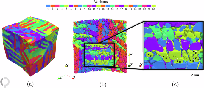
a Full simulation domain showing overall martensite structure. b 2D side view with transparent interfaces. c Zoom-in view outlined by the black box, demonstrating blocks’ composition of different sub-blocks, represented by a distinct martensite variant color where shades of the same color represent K-S variants stemming from the same Bain variant.
The stress evolution correlated with these transformations revealed an inverse relationship between the plastic slip rate and the residual stresses as illustrated in Fig. 4 where higher plastic slip rates lead to lower residual stresses, and vice versa. The highest slip rate, 1 × 10⁻² s−1, coincided with the earliest onset of martensitic transformation and the lowest residual stress at 1.8 GPa, indicating efficient plastic accommodation of the transformation-induced deformation. In contrast, the lowest slip rate of 1 × 10⁻⁶ s−1 exhibited the highest residual stress of ~5.2 GPa due to the inability to promptly relax the transformation-induced deformations, which is an important observation in our simulations.
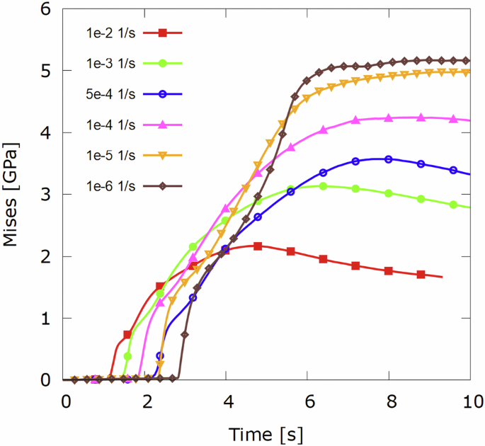
Evolution of average von Mises stress over time during martensitic transformation at different plastic slip rates (1×10⁻² to 1×10⁻⁶ s⁻¹). Lower slip rates result in higher residual stresses, with peak values ranging from 1.8 GPa to 5.2 GPa.
Effect of heat extraction rate on transformation kinetics
In order to investigate the effects of heat extraction rate on the kinetics of martensitic transformation a set of simulations at different heat extraction rates were conducted for a steel grade containing 0.1 wt.% carbon. The chosen heat extraction rates correspond to 100 K/s, 200 K/s, and 400 K/s effective cooling rate at the onset of the transformation. Increasing the effective cooling rate by factors 2 and 4 required decreasing the simulation time step by the same factors while adjusting the plastic slip rates respectively to 5 × 10⁻⁴, 2 × 10⁻³ and 8 × 10⁻³ s−1 to compensate for the change in effective deformation increment in each simulation time step. The plastic slip rates used in this study (5 × 10⁻⁴, 2 × 10⁻³, 8 × 10⁻³ s−1) were selected to maintain a consistent ratio between the effective plastic relaxation rate and the effective cooling rate. Due to the increased transformation rate for higher cooling rates, the time step of the simulations had to be reduced by a factor of 2 to maintain simulation stability. At the same time, our plasticity model is time increment sensitive, requiring a factor 2 slip rate increase to compensate for the reduced time step. This resulted in a factor 4 instead of 2 increase in the plastic slip rate. Such a slip rate adjustment ensures that the relative rates of transformation and plastic accommodation are comparable across different cooling conditions, allowing for a systematic investigation of their interplay.
To maintain consistency across different cooling rates, we also adjusted the interface mobility (kinetic coefficients Mαβ in Eq. (5)) in addition to the plastic slip rates and simulation time steps. Table 2 summarizes these adjustments.
These adjustments ensure that the relative rates of transformation and plastic accommodation are comparable across different cooling conditions, allowing for a systematic investigation of their interplay. The increase in mobility for higher cooling rates compensates for the reduced time steps, maintaining the overall transformation kinetics relative to the cooling rate.
The volume fraction plots in Fig. 5 show that a more rapid quench leads to a higher volume fraction of martensite at any given temperature. This is related to the behavior of the transformation-induced stress which is shown in Fig. 6 for different cooling rates. The results demonstrate that as the cooling rate increases, the martensite transformation starts to occur earlier and proceeds more rapidly, initially leading to higher internal stresses. However, the transformation-induced stresses are significantly influenced by the adjusted slip rates. Thus, the final saturated stress levels were notably higher for lower cooling rates and correspondingly lower slip rates. This counter-intuitive result indicates that at slower cooling rates, despite the reduced rate of martensite formation, the slower plastic relaxation fails to relieve the transformation-induced stresses efficiently. Such behavior is attributed to the limitations of the modeling approach used in this study where rate dependence of the phenomenological crystal plasticity model interferes with the martensite growth kinetics at the time scale of the cooling process.
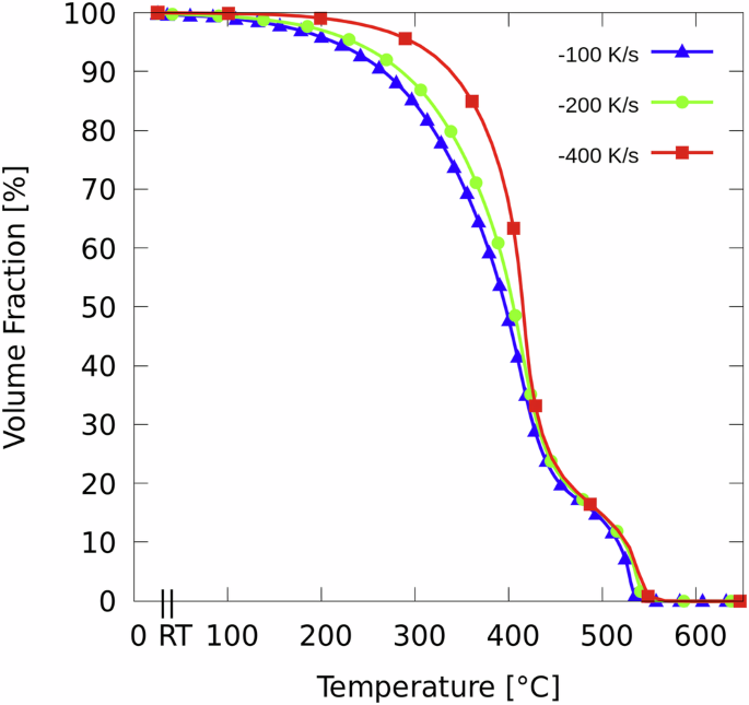
Temperature-dependent evolution of martensite volume fraction during continuous cooling at rates from −100 K/s to −400 K/s. Higher cooling rates promote earlier transformation onset and faster transformation kinetics. Room temperature (RT) is indicated on the temperature axis.
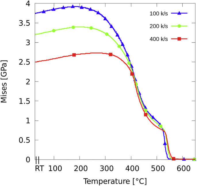
The temperature evolution of von Mises stress during martensitic transformation at cooling rates from 100 K/s to 400 K/s shows that counterintuitively, slower cooling rates result in higher peak stresses due to reduced plastic relaxation efficiency.
Effect of carbon content on phase transformation
The effect of carbon content on the martensite formation kinetics has been investigated by performing the simulations for steel grades with three different carbon concentrations for various carbon concentrations: 0.1, 0.2, and 0.3 wt.%. The simulations have been performed at a constant plastic slip rate of 5 × 10⁻⁴ s−1 and an effective cooling rate of 100K/s. Such simulation setup allows us to study the interplay between the thermodynamic driving force controlled by the carbon content, the mechanical accommodation of transformation-induced deformations which differs for different carbon content, and plasticity model hardening due to lower transformation temperature for higher carbon content steel grades. The volume fraction evolution shown in Fig. 7 demonstrates a clear sensitivity of the martensite start temperature, Ms, to the carbon content, where higher carbon concentration leads to lower martensite start temperature. The stress profiles shown in Fig. 8 demonstrate similar stress levels during the transformation for different carbon contents. The average plastic strain evolution for different carbon content (see Fig. 9) shows slight increase with increased carbon content due to increased transformation-induced deformation (see Table 4 for the reference).
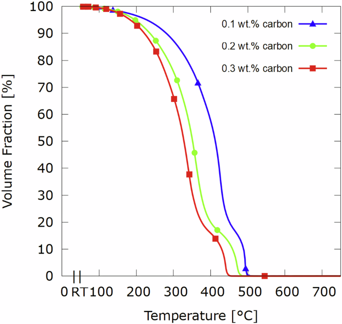
Temperature-dependent evolution of martensite volume fraction for steels containing 0.1–0.3 wt.% carbon. Higher carbon content results in lower martensite start temperatures, from room temperature (RT) to 700 °C.
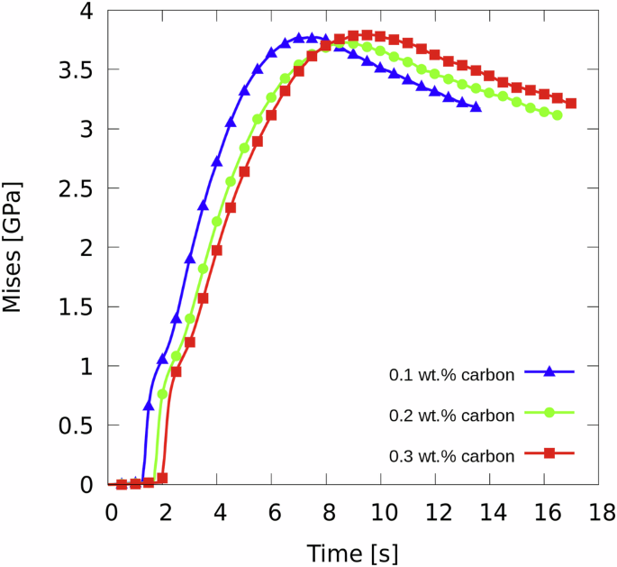
Time-dependent von Mises stress development during transformation for 0.1–0.3 wt.% carbon steels, showing similar peak stress levels (~3.8 GPa) but different evolution patterns.
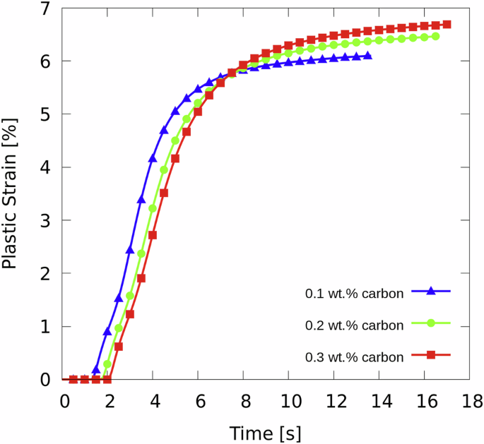
Time evolution of average plastic strain for different carbon contents (0.1–0.3 wt.%), showing increased final strain values with higher carbon content.
In studying the martensitic transformations in steel the experimental dilatometry curves are crucial in understanding the kinetics of martensite formation. They help to investigate the martensite start and finish temperatures and the martensite volume fraction evolution over temperature using relatively simple measurement technique. The method is based on measuring the sample length change due to the thermal contraction and the volumetric expansion due to the austenite-to-martensite transformation. To accurately model dilatometry curves, we employed an approach that accounts for the temperature-dependent thermal expansion of both austenite and martensite phases, as well as the transformation-induced deformation (for details see “Dilatometry Curve Modeling”). Fig. 10 shows that at the martensite start temperatures deduced from the volume fraction evolution, the dilatometry curves exhibit a notable increase in length change. The simulated martensite start temperatures (({M}_{s}^{sim})) of 497 °C, 465 °C, and 446 °C for 0.1, 0.2, and 0.3 wt.% carbon, respectively, align closely with experimental values (see Table 3). Furthermore, it has been noted that increasing carbon content leads to a significant increase in length change upon further cooling, which is attributed to the higher transformation-induced lattice parameter change for higher carbon content, as reflected in the Bain strain components used in the calculation (see Table 4). This trend in length change with respect to carbon content is consistent with experimental observations and theoretical predictions for martensitic transformations in low-carbon steels.
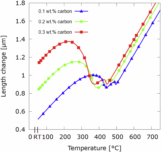
Temperature-dependent length change during transformation, showing increased dimensional changes with higher carbon content and distinct transformation start temperatures (Mssim) of 497 °C, 465 °C, and 446 °C for 0.1, 0.2, and 0.3 wt.% carbon, respectively.
The simulated martensite start temperatures (({M}_{s}^{sim})) of 497 °C, 465 °C, and 446 °C for 0.1, 0.2, and 0.3 wt.% carbon, respectively, show general agreement with experimental values, particularly for lower carbon contents. While some deviations are observed, especially at higher carbon concentrations, the overall trend and resulting microstructural features align well with the experimental and theoretical findings reported in47. It is important to note that the simulated Ms temperatures are influenced by the interplay between the transformation rate and the rate of plastic relaxation in our model. Consequently, they should be interpreted as representing a range of temperatures where martensite formation becomes favorable, rather than precise values.
The simulated microstructures for different carbon content are shown in Fig. 11. All three microstructures show a regular combination of 24 Kurdjumov-Sachs variants in a lath-like arrangement similar to the microstructures reported in literature65,66,67 and can be used as realistic representative volume elements for further mechanical testing.
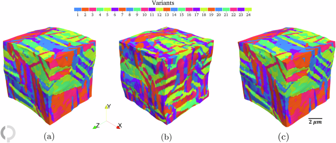
a 0.1 wt.%, b 0.2 wt.%, and c 0.3 wt.%. All simulations were performed at a constant plastic slip rate of 5 × 10⁻⁴ s−1 and an effective cooling rate of 100 K/s. Colors represent the 24 Kurdjumov-Sachs orientation variants.
Discussion
The present study provides new insights into the complex interplay between martensitic transformation and plastic relaxation rates in low-carbon steels. Advanced phase-field simulations coupled with a full-featured finite strain crystal plasticity model enabled systematic investigation of the interplay between plastic deformation rate, heat extraction rate, and carbon content on transformation kinetics, microstructure formation and internal stresses evolution. The underlying mechanism, as hypothesized, is the competition between the rapid martensitic transformation driven by thermal undercooling and the inherently slower process of plastic relaxation. Martensite, forming almost instantaneously and straining the surrounding matrix by 20%, rapidly reaches a mechanical energy barrier where the high local stresses counterbalance the chemical driving force, arresting further transformation. Only upon additional cooling does the material overcome this mechanical barrier, as the accrued chemical energy surpasses the mechanical resistance, allowing transformation to proceed.
The transformation-induced deformation and the resulting plastic relaxation occur locally at time scales significantly faster than the cooling process and thus pose significant limitations on the phase-field modeling. Our simulations bridge this gap by adjusting the plastic slip rate and aligning the rate of plastic relaxation with the rate of heat extraction which drives the overall transformation kinetics at the mesoscale. This approach enables us to simulate a transformation process that maintains a proportional relationship between the transformation rate and the rate of plastic relaxation while being away from the true speeds of sound or the true deformation rates of martensitic transformation. The arrangement and orientation of the observed microstructures suggest that plastic relaxation, though slower than the transformation-induce deformation, is an essential factor in determining the final morphology of martensite. Our results demonstrate that there exist a significant time scale difference between the rate of transformation-induced deformation and the resulting plastic relaxation. Mapping this time scale difference back to the atomistic time and space scales such time scale difference can be attributed to the kinetics of dislocations generation necessary to accommodate the growing martensite laths which is significantly slower than the speed of transformation-induced deformation propagation, i.e., the speed of sound in steel. Here, in line with the slipped martensite formation picture68, we assume that considering around 20% characteristic deformation inherent to the martensitic transformation a single dislocation loop can be introduced every 5 atomic layers of austenite to fully accommodate such deformation. Thus, significant dislocation generation in prior austenite grain at the martensite growth front has to take place during the growth of individual martensite laths.
In summary, our simulations reveal several key findings:
-
A critical threshold in the plastic relaxation rate exists, below which the steel’s intrinsic capacity for plastic deformation lags behind the rapid martensitic transformation. This leads to a transition from the formation of finer uniform microstructure at higher plastic slip rates to elongated lath-like martensite structures at lower slip rates.
-
The stress evolution exhibits an inverse relationship with the plastic slip rate, with slower plastic relaxation resulting in higher residual stresses.
-
The heat extraction rate plays a crucial role in the transformation kinetics, with faster heat extraction rates leading to higher martensite start temperatures and more rapid transformation kinetics. However, the ability to accommodate the transformation-induced stresses depends on the delicate balance between the heat extraction rate and the rate of plastic relaxation.
-
Carbon content emerges as a key factor in the phase transformation behavior, with higher carbon levels stabilizing the austenite phase and delaying the martensite start temperature. The simulated dilatometry curves and microstructures accurately capture the influence of carbon content, aligning closely with experimental observations.
In conclusion, our findings contribute to a deeper understanding of the complex kinetics of martensitic transformation in low-carbon steels. The study suggests that the interplay between the rapid transformation at sonic speeds and the slower plastic accommodation is fundamental to understanding the martensite microstructure formation process. The apparent competition between the rapid transformation and the requirement for plastic deformation challenges traditional notions and opens new avenues for further investigation into the kinetics of phase transformations in steel. The advanced modeling approach and comprehensive analysis of the interplay between the transformation and plastic relaxation rates provide valuable insights for material scientists and engineers developing high-performance steels.
Methods
Phase-field method
In this study the multi-phase-field (MPF) framework35,69,70 coupled to the phenomenological crystal plasticity model71 is utilized to investigate the martensitic microstructure formation in low-carbon steel. The MPF model can treat a virtually unlimited number of grains using a set of phase-field variables, ϕα(x, t), as functions of spatial coordinates and time, where α is the running index of the grain allowing to assign different properties and orientation to each grain. The phase-field parameters values are ranging between 0 and 1, where the value of 0 indicates being outside of the grain, and 1 indicates being inside of the bulk of the grain with a smooth transition between 0 and 1 indicating the diffuse interface between the grains. The sum over all phase-field variables in every point in space is constrained:
The time evolution equation of the phase-field parameter is constructed as a sum over all dual interactions between the grains70:
where ({M}_{alpha beta }^{phi }) is the grain boundary mobility, defined separately for each pair of grains, N is the number of non-zero phase fields present in a given point, η is the interface width, and F is the total free energy of the system. (frac{delta }{delta {phi }_{alpha }}) denotes functional derivative operator with respect to the phase-field variable ϕα.
The total free energy functional, F, in the MPF model is described as an integral of different free energy density contributions within the material volume Ω (for a detailed explanation see72). For martensitic transformation, we restrict our consideration to the interface free energy density, f intf, the mechanical free energy density, f mech, and the chemical free energy density, fchem:
The interface free energy density using the double obstacle interface potential is expressed as follows:
where σαβ is the interface energy between the two grains (or phases) α and β.
The resulting phase-field evolution equation has the form
where ({I}_{gamma }={nabla }^{2}{phi }_{gamma }+frac{{pi }^{2}}{{eta }^{2}}{phi }_{gamma }) is the generalized curvature, Δgαβ is the driving force depending on the bulk energy difference (chemical and mechanical) between the two grains (or phases) α and β.
The chemical free energy density is modeled as an algebraic mixture of the bulk free energy densities of the individual phases as function of temperature and their phase composition, ({vec{c}}_{alpha }), weighted by the corresponding phase fields:
Additional factors require careful consideration in addressing the mechanical free energy density. It is well established that the effective mechanical characteristics of a composite material, consisting of multiple phases, are influenced by both the phase distribution and the load direction. The theoretical framework for formulating an effective description of these material properties is termed ”homogenization”. The Voigt-Taylor and Reuss-Sachs models within this framework represent two distinct extremes. The application of these concepts to phase-field models, particularly in relation to interfaces conceptualized as composites of two phases (or multiple phases in multi-junctions), was initially examined in73. Present understanding endorses the rank-1 convexification model74, which serves as an intermediary between these extremes by simultaneously ensuring the force balance and kinematic compatibility at the interface. This is further substantiated by references such as75,76,77. However, owing to the computational complexity inherent in this approach, in particular the lack of closed form solution for junctions between more than two grains or variants, the current work is limited to the Khachaturyan’s elasticity model and we leave closer consideration of rank-1 convexification for future work.
The mechanical free energy density is defined using the St. Venant-Kirchhoff hyperelastic model and has the form
where Eel is the Green-Lagrange elastic strain tensor and (hat{{bf{C}}}) is the effective elasticity tensor, both subject to proper homogenization or elasticity model consideration. In the current study Khachaturyan’s elasticity model78 is considered due its numerical efficiency resulting in the following definition of the elasticity tensor
where ({hat{{bf{C}}}}_{alpha }) are the elasticity moduli of the individual grains or phases.
The general form of the mechanical equilibrium condition in the absence of external forces has the form
where P = F S is the first Piola-Kirchhoff stress tensor and S is the second Piola-Kirchhoff stress tensor defined in the reference configuration.
The elastic deformation gradient tensor is defined using the multiplicative decomposition of the deformation gradient tensor
where Fel is the elastic deformation gradient tensor, Fpl is the plastic deformation gradient tensor and ({{bf{F}}}_{{rm{tr}}}) is the transformation-induced deformation gradient tensor.
The transformation-induced deformation gradient tensor is given by
where ({{bf{F}}}_{{rm{tr}}}^{alpha }) are the transformation-induced deformations of individual phases or grains α. For convenience, the transformation-induced deformations are defined taking the matrix phase as the reference. The definition of the plastic deformation gradient tensor, Fpl, is given in 3.2.
The elastic Green-Lagrange finite strain tensor reads
where
is the elastic deformation gradient tensor.
The elastic second Piola-Kirchhoff stress tensor in the intermediate configuration, obtained after the transformation induced and/or plastic deformation, has the form
Then, the second Piola-Kirchhoff stress tensor in the reference configuration suitable for the mechanical equilibrium calculation in Eq. (9) can be obtained via the pull back operation
where ({J}_{{rm{tr}}}) is the Jacobian of the transformation-induced deformation gradient tensor ({{bf{F}}}_{{rm{tr}}}).
Substituting Eq. (15) into Eq. (9) the updated mechanical equilibrium equation reads
The three Bain stretch tensors79 which are related to three orthogonal tetragonally distorted crystal structures are given by
Following79, the components of the Bain stretch tensors above for the FCC (austenite) to BCC/BCT (martensite) transformation read
where aA is the lattice parameter of the FCC austenite, aM and cM are the lattice parameters of the BCC/BCT martensite. In order to determine the components of the Bain stretch tensor, the lattice constants of austenite and martensite are used at the temperature corresponding to Ms temperature for three different carbon concentrations. This calculation is done in accordance with ref. 80. In this study we consider three different carbon compositions, and the computed Bain stretches for each of them are presented in 4.
The composition dependent stiffness parameters of the austenite and martensite phases in this study are taken from ref. 47. The stiffness tensors of all 24 K-S martensite variants are obtained by applying the rotation matrices, Oi (i = 1, 2, … , 24), corresponding to the K-S OR between the austenite and martensite, to a single tetragonal Bain variant U3. In general, the OR is given through the matrix:
where the R[−45°, ei] = R[90°, ei]R[−45°, ei] with ({bf{R}}[9{0}^{circ },{e}_{i}]in {{mathcal{P}}}_{24}), i.e., selecting the opposite sign for the 45° rotation about ei simply leads to a crystallographically equivalent normal and direction. The tranformation-induced rotation matrices Ri in Eq. (18) are derived from the combination of rotations around specific crystallographic axes defined by:
where θ(r) and ϕ(r) are the rotation angles given by:
where (r=c/a=sqrt{2}{U}_{c}/{U}_{a}) is the ratio of tetragonality of the BCT cell.
The transformation-induced deformation gradient tensor for the i-th K-S variant is given by81:
where Uj, (j = 1, 2, 3) is one of the Bain stretch tensors.
For the specific case of the KS1 variant (assuming r = 1 for BCC), we have θ(1) ≈ 5.2644° and ϕ(1) ≈ 9.7356°. Thus, the OR matrix OKS1 between the austenite and the first K-S variant of martensite is given by
and the resulting transformation-induced deformation gradient tensor reads
Given a transformation-induced deformation gradient Ftr,KS1 we are able to generate further variants through the application of ({{mathcal{P}}}^{24}) point group. Thus, the remaining 23 K-S variants are given by
or, in short form,
where Pj, are the elements of the ({{mathcal{P}}}^{24}) point group.
The stiffness tensors of all martensite variants can be obtained following the same procedure starting from the stiffness tensor of KS1 variant of martensite.
Crystal plasticity model
In this study the plastic deformation accompanying the martensitic transformation is modeled using the phenomenological crystal plasticity model30. Within this model the evolution of the plastic deformation gradient ({dot{mathbf{F}}}_{{rm{pl}}}) is given by
where Lpl is the plastic velocity gradient tensor given by
where ({dot{gamma }}_{alpha }^{t}) is the shear rate on each slip system t and ({{bf{M}}}_{alpha }^{t}) is the non-symmetric Schmid tensor corresponding to each grain or phase α. The Schmid tensor is calculated as follows
where ({{bf{m}}}_{alpha }^{t}) represents the slip direction vector and ({{bf{n}}}_{alpha }^{t}) is the normal to the slip plane of individual slip systems t considering the symmetry and the orientation of the grain. The shear rate on the slip system t is formulated as a function of the resolved shear stress τt, obtained from the elastic second Piola-Kirchhoff stress in the intermediate configuration, Sel, and the critical resolved shear stress (CRSS) ({tau }_{c,alpha }^{t}) in each grain or phase α:
where ({dot{gamma }}_{0,alpha }) determines the reference shear rate and n is the rate sensitivity parameter.
The evolution of CRSS is a key parameter in the plastic deformation behavior of a material and is governed by the hardening law:
where τs,α is the saturation stress, representing the maximum attainable critical resolved shear stress for a given material, h0 is the hardening modulus, indicating the initial hardening rate, ({q}_{alpha }^{t,u}) is the latent hardening ratio between slip systems t and u. When t = u, it represents the self-hardening, while for t ≠ u, it represents cross-hardening (interaction between slip systems). m is the hardening exponent parameter, controlling the rate at which hardening occurs.
In order to use the phenomenological crystal plasticity model, the initial step requires gathering plasticity data for both austenite and martensite within the temperature range of the transformation. However, this endeavor is quite demanding due to the thermodynamic instability of austenite (FCC-Iron) at low temperatures, which makes it challenging to conduct corresponding tests at the martensite formation temperatures. Additionally, there are no current plasticity models for the martensite’s BCT structure. Adopting the BCC model facilitates the examination of martensite formation without hindering the analysis. Table 5 gives the list of FCC and BCC slips systems used in this study. Table 6 summarizes the crystal plasticity parameters that were used for both austenite and martensite in this work.
Transformation driving force
The martensitic transformation in low carbon steel is characterized by its lack of thermal activation. The chemical part of the thermodynamic driving force of the transformation can be described through the difference in Gibbs free energy between the parent phase (austenite) and the product phase (martensite), a value which, considering suppressed carbon diffusion, is only dependent on temperature82:
where Δg(T) denotes the thermodynamic driving force at temperature T, T0 represents the equilibrium temperature at which the Gibbs free energies of austenite and martensite are equal, and Q is the latent heat associated with the austenite-to-martensite phase transformation. The equilibrium temperature T0 is obtained via Thermo-Calc simulations, while the latent heat Q is calculated based on a subsequently introduced empirical formula.
At the onset of martensite formation, identified as the martensite start temperature (Ms), the Gibbs free energy difference reaches a critical value necessary for the transformation. The nominal alloy composition dependence of the critical thermodynamic driving force has been proposed by Cool and Bhadeshia83. The expression for the critical driving force, tailored to the steel grades considered in this study, reads
Integrating both equations with the experimental ({M}_{s}^{exp}) values, we determined the equivalent latent heat value Q for the low-carbon steel samples analyzed in this study. Table 7 presents a summary of these thermodynamic parameters.
To conduct a realistic simulation involving the heat extraction process during quenching, we used Newton’s law of cooling and incorporated the effect of latent heat release as follows
where T(t) is the temperature of the sample which is assumed isotropic, Ts is the temperature of the cooling medium, (k=frac{A}{V}frac{alpha }{rho {c}_{p}},,[frac{1}{s}]) is the simplified heat extraction coefficient which depends on the surface to volume ratio (frac{A}{V}) and the heat transfer coefficient α between the sample and the cooling medium normalized by the heat capacity of the material ρcp. The heat extraction coefficient allows to consider different cooling media, e.g., air, oil or water. (dot{f}) denotes the rate of phase change, averaged over the sample volume.
Dilatometry curve modeling
To accurately model the dilatometry curves associated with martensitic transformation, we employed an approach that accounts for the thermal expansion of both austenite and martensite phases, as well as the transformation strain. This model allows us to simulate the length changes observed during experimental dilatometry measurements.
The length change as a function of temperature and martensite fraction is calculated using the following equation:
where
-
ΔL(T, fM) is the length change at temperature T,
-
L0 is the initial length (12.8 μm in our simulations),
-
Tref is the reference temperature set to Ms for different carbon content,
-
αA is the thermal expansion coefficient of austenite,
-
αM is the thermal expansion coefficient of martensite,
-
T is the temperature in Kelvin,
-
fM is the martensite volume fraction,
-
αtr is the transformation-induced deformation.
The composition-dependent thermal expansion coefficients for austenite and martensite are given by:
where cA and cM denote the mole fraction of carbon in austenite and martensite, respectively80.
The transformation-induced deformation αtr is calculated based on the Bain stretch tensor components:
where Ua and Uc are the diagonal Bain stretch tensor components, which depend on the carbon content of the steel (see Table 4).
This model allows us to simulate the dilatometry curves for different carbon contents and cooling rates, providing additional information on the martensitic transformation kinetics. The simulated dilatometry curves can be directly compared with experimental dilatometry data, offering an additional tool for validating the phase-field simulations.
Calibration of the plasticity model of austenite
In this study, we conducted a series of deformation simulations using the crystal plasticity model of austenite to calibrate the temperature-dependent phenomenological crystal plasticity model parameters taking the results from ref. 84 as the reference. The deformation simulations focus on determining austenite’s yield strength in isolation, with flow stress responses plotted for various temperatures, capturing deformation up to 10% (see Fig. 12). The resulting plot shows a clear temperature dependence of the flow stress of austenite. The trend is consistent with the known behavior, where higher temperatures lead to lower yield strength of austenite. A noteworthy aspect of the deformation test results is the model’s ability to capture austenite’s mechanical behavior at different temperatures where the simulation data closely aligns with the experimentally measured results. The values obtained in these test simulations were used in the modeling of the martensitic transformation for steel grades with different carbon content which show different martensite start temperature and thus different austenite yield strength at the onset of the transformation.
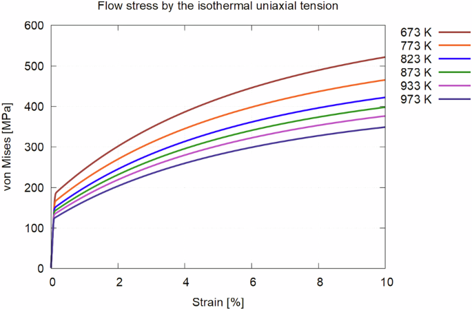
(von Mises is calculated from the second Piola-Kirchhoff stress tensor).
Improved finite strain elasticity model
In the current study, we utilized a newly developed finite strain elasticity solver59 integrated into the phase-field method, which allows us to address the complex mechanical behavior associated with large transformation-induced deformations during martensitic transformation. One of the important aspect of the micro-mechanical modeling of the martensite formation in steel is rigorous consideration of the transformation-induced local lattice rotations responsible for the formation of 24 K-S variants instead of only 3 Bain variants of martensite. This has been largely overlooked in literature till present. The use of the newly developed elasticity solver allows us to fully account for the local lattice rotations induced by the transformation which is a significant step forward in modeling the masrtensitic transformations in steel.
Figure 13a shows one of the simulated martensite microstructures displaying all 24 K-S variants within a single grain. The local lattice rotations derived from the deformation gradients are shown in Fig. 13c. The displayed rotation angles are obtained via the polar decomposition of the local deformation gradient tensor into pure stretch and pure rotation and then converting the rotation tensor into the axis-angle representations. The results demonstrate local lattice rotations up to 25° which is in line with the typical lattice rotations stemming from the martensitic transformation composed of around ±10° rotation around the (110) axes and ±5° around the (111) axes. The simulation domain deformation is shown in Fig. 13b indicating significant surface relief typically observed in light optical microscopy studies.
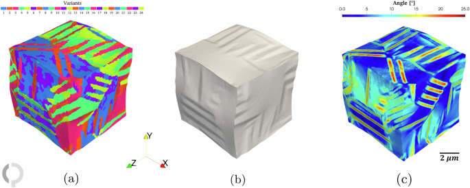
a Three-dimensional representation of martensite variants showing all 24 Kurdjumov-Sachs orientation relationships within a single prior austenite grain, colored according to variant number, (b) simulated surface relief pattern showing characteristic topographical features of martensitic transformation, and (c) local lattice rotation map showing rotation angles up to 25°, with rotations around (110) axes of ±10° and (111) axes of ±5°.


Responses