The logarithmic memristor-based Bayesian machine

The rapid evolution of artificial intelligence (AI) applications at the edge has accentuated the demand for low-power, explainable, and reliable edge AI systems that can function effectively even in uncertain conditions¹. Numerous works have shown that advanced memory devices allow for considerable energy savings for the implementation of neural networks, a non-explainable form of AI, through the cointegration of computation and memory^2,3,4,5,6. This cointegration can also be applied to explainable AI, as exemplified by the recently demonstrated nanodevice-based Bayesian machines^7,8. Relying on Bayesian inference^9,10, the strengths of these machines are manifold: they provide a hardware AI with inherently explainable results^11,12, at a high energy efficiency. Bayesian machines are particularly appealing for tasks where neural networks struggle, such as sensor fusion in highly uncertain environments with limited training data, or safety-critical applications requiring explainable decisions.

The efficiency of Bayesian machines is achieved through near-memory computing, which offsets the high cost of accessing the parameters of the Bayesian model¹³, and the adoption of stochastic computing^14,15. The latter particularly facilitates compact and energy-efficient multiplication, a dominant arithmetic operation in the Bayesian machine, and has been shown repeatedly to be particularly adapted to Bayesian inference^{16,17,18,19,20,21,22,23,24}. Despite all their merits, Bayesian machines are not exempt from the challenges of stochastic computing. These include high latency and compromised precision when dealing with low probability values^15,25. While Bayesian machines demonstrated high accuracy in a gesture recognition application⁷ or on handwritten character recognition⁸, their broader applicability to diverse tasks remains an open question.

Our contribution through this work is two-fold. First, we introduce an alternative design: the logarithmic memristor-based Bayesian machine. This design eschews stochastic computing in favor of logarithmic computing²⁵. This modification translates to implementing probability multiplications using digital near-memory integer adders, thereby augmenting the versatility of the system. We present a fully fabricated logarithmic Bayesian machine, using a hybrid CMOS/hafnium-oxide memristor process and show its robustness experimentally. Second, we undertake a comprehensive evaluation of this machine for gesture recognition and also for a Bayesian filter application that addresses a time-dependent task: sleep stage classification throughout the night. A detailed comparison with the stochastic design, assessing accuracy and energy consumption, elucidates the scenarios in which each design excels.

Preliminary measurements of the logarithmic Bayesian machine were presented at recent conferences^26,27. This paper builds on additional measurements and simulations, providing extensive comparisons between the logarithmic and stochastic versions of the Bayesian machines.

Bayesian machines: the logarithmic approach

The primary objective of a Bayesian machine is performing the inference of Bayesian models, specifically Bayesian networks. Its versatile nature allows adaptation to various model types. The general concept of Bayesian inference is to estimate the probability of a variable Y based on observations O_i using Bayes’s law

where p(Y = y) is our prior belief on the variable to infer, and p(O₁, O₂, …, O_n) acts as a normalization constant. The likelihood of the observations p(O₁, O₂, …, O_n∣Y = y) constitutes the core of the Bayesian model. Its size on a discrete k-symbol observation space grows exponentially as kⁿ, making exact Bayesian inference impractical and intractable. Therefore, independence assumptions based on expert knowledge are commonly applied, typically within the framework of Bayesian networks.

The strongest simplification is called naive Bayesian inference, where we assume that observations are conditionally independent, meaning ∀i, j, p(O_i, O_j∣Y = y)= p(O_i∣Y = y)p(O_j∣Y = y). This allows us to write

The likelihoods p(O_i∣Y = y), as well as the priors p(Y = y) constitute the parameters of the model. We do not need to compute the normalization constant, as it is sufficient and simpler to normalize across all y values after an inference.

More complex, non-naive models can also be represented similarly. For example, if observations O₂ and O₃ cannot be considered conditionally independent, they can be grouped, allowing us to write

Our Bayesian machines allow computing equations like Eqs. (2) and (3) using near-memory computing, thereby achieving substantial energy savings. They all use the topology presented in Fig. 1a: the priors and likelihoods are stored in memory arrays, the observations are presented by vertical wires, and the posterior is computed near memory, sequentially on horizontal wires. Figure 1a is presented in the naive Bayesian inference case (Eq. (2)). In the non-naive case (Eq. (3)), non-conditionally independent observations would be presented on adjacent, vertical wires (see Supplementary Note 1 of ref. ⁷).

a General schematic of the computations of a Bayesian machine. b, c Simplified schematic of the implemented logarithmic and stochastic Bayesian machines. All log-probabilities in the logarithmic machine are coded as eight-bit integers, following Eq. (4).

Full size image

The different Bayesian machine designs differ in how they store likelihoods and priors and in their methods of computing the product of probabilities. In the stochastic Bayesian machine (Fig. 1c), stochastic computing is employed to compute the product of probabilities in equations such as Eq. (2). All probability values are represented by a stochastic bit stream whose probability of being one is the coded probability. Then, multiplication is achieved with great energy efficiency and compactness by utilizing only AND gates^7,14,15. However, the stochastic machine possesses inherent challenges. First, it needs random number generators (RNGs). While these RNGs can be shared column-wise to mitigate their cost, energy is spent for transmitting the random numbers throughout the column. Second, when likelihoods are small, stochastic computing can require an unreasonably high number of clock cycles to provide accurate results¹⁵.

In this work, we introduce the logarithmic Bayesian machine (Fig. 1b), where we explore an alternative approach, which transforms products into sums. All probability values are represented logarithmically using integers. The correspondence between a real probability p and the integer n is

Throughout our research, we used 8-bit integers to represent n, and we selected B = 1/2 and m = 8. This encoding implies that integer values from 0 to 8 correspond to probabilities ranging between 1 and 1/2, while values from 9 to 255 represent probabilities smaller than 1/2. The smallest probability that can be coded is ({frac{1}{2}}^{255/8}approx 2.5times 1{0}^{-10}). Therefore, this encoding prioritizes lower probability values, contrasting with the methodology of stochastic computing, where such values are difficult to process. While similar logarithmic representations have been employed in general-purpose computing contexts^25,28,29, this specific representation has not been previously applied to Bayesian inference.

Our logarithmic Bayesian machine, as depicted in Fig. 1b, retains the architectural principle of its stochastic counterpart. Memristor arrays host logarithmic integer representations of the likelihoods p(O_i∣Y = y), with storage as 8-bit integers. The input observations O_i provide row addresses for these arrays, indicating the specific likelihood value to access. These values are then aggregated using near-memory 8-bit integer adders, which substitute the 1-bit AND gates found in the stochastic model. Our adders are designed to yield a 255 output (i.e., the minimum possible probability) in overflow scenarios.

Sleep stage classification using a fabricated hybrid memristor/CMOS logarithmic Bayesian machine

Employing a hybrid CMOS/memristor process, we fabricated a logarithmic Bayesian machine test chip (Fig. 2). The memristors, also referred to as resistive RAM, ReRAM, or RRAM in industrial contexts, comprise a stack of titanium nitride, hafnium oxide, titanium, and titanium nitride. A detailed overview of the process is presented in the “Methods” section. Figure 2a–c displays optical images of the die, which includes 16 memristor array blocks. Its layout closely aligns with the general topology shown in Fig. 1b. The memristors are embedded in the backend of the line of the CMOS, positioned between metal levels four and five, as illustrated in the electron microscopy image of Fig. 2d.

a Optical microscopy image of the die of the fabricated machine. b Detail of the likelihood block, which consists of digital circuitry and memory block with its periphery circuit. c Photograph of the 2T2R memristor array. d Scanning electron microscopy image of a memristor in the back end of the line of our hybrid memristor/CMOS process.

Full size image

Despite their functionality, memristors are not flawless. Their imperfections can lead to bit errors, which are eliminated using strong error correction codes (ECC) in industrial designs^30,31. In our design, we use an alternative approach. To counteract errors emerging from memristor variability³² and instability³³, we have used a two-transistor/two-memristor (2T2R) bit cell configuration (Fig. 3a). In this cell, bits are programmed complementarily. This technique, adopted previously in the stochastic Bayesian machine⁷ and in a memristor-based binarized neural network³⁴, has demonstrated a marked reduction in bit error rate, rivaling the efficiency of a single-error-correction, double-error-detection (SECDED) ECC with equivalent redundancy³⁵. This efficiency is seen in the experimental results of Fig. 3c, showing results from previous work³⁵ obtained using a 1024 memristor array of the same process as the logarithmic Bayesian machine. The 2T2R cells are read using precharge sense amplifiers (PCSA)^36,37 (Fig. 3b). Each column of the memristor array features its dedicated sense amplifier.

a Schematic of the likelihood block is presented in Fig. 2b. b Schematic of the differential pre-charge sense amplifier (PCSA) used to read the binary memristor states. c Error rate of the 2T2R approach as a function of the error rate of the 1T1R approach. The different points are obtained by varying memristor programming conditions on a 1024-memristor array (results reproduced from ref. ³⁵, see main text). d Schematic of the level shifter. e Cumulative distribution function of the resistance of memristors for the two programmed states: low resistance state (LRS) and high resistance state (HRS), measured on a 1024-memristor array (see the “Methods” section).

Full size image

The test chip also houses comprehensive control circuitry for programming the memristors (detailed in the “Methods” section). In particular, rows and columns periphery circuitry include level shifters (Fig. 3d) that are used solely during memristor write operations to raise the voltage from the logic nominal voltage to higher-than-nominal voltages able to write the memristors (see the “Methods section). Figure 3e shows the cumulative distribution functions of the resistance of memristors programmed in low and high resistance states with the programming conditions in the logarithmic Bayesian machines (see the “Methods” section). The ratio between the mean value of the high resistance state distribution and the mean value of the low resistance distribution is equal to 28.2, whereas the minimum ratio at three sigmas is equal to 1.35. Note that these measurements were performed on a different circuit than the logarithmic Bayesian machine, allowing direct access to the memristors.

We have thoroughly probe tested the Bayesian machine, aided by a specialized printed circuit board that facilitates comprehensive computer control, presented in Fig. 4d (see the “Methods” section).

a Inputs and and outputs of the logarithmic Bayesian machine used for sleep stage classification. b Bayesian network model implemented on the logarithmic Bayesian machine used for sleep stage classification. c Experimentally measured test accuracy of the logarithmic Bayesian machine, averaged over 1000 five-second segments. The measurement was repeated for various supply voltages VDD. d Photograph of the experimental setup.

Full size image

In this study, we have employed sleep stage classification throughout the night as a benchmark task to evaluate our integrated circuit. Mathematically, this task is more intricate than the gesture recognition task used for evaluating the stochastic Bayesian machine in ref. ⁷. A typical night’s sleep comprises different stages: awake, rapid eye movement (REM), light sleep, and deep sleep. Note that for simplicity, we have aggregated “light” and “deep” sleep stages, which are sometimes each separated into two separate stages (refer to the “Methods” section for details). Our objective is to classify sleep stages throughout the night using electroencephalography (EEG) and electromyography (EMG) measurements.

Inferring sleep stages solely from EEG and EMG readings is challenging. The temporal context plays a crucial role: if a patient is identified to be in deep sleep at time t, the likelihood of the same stage five seconds later (denoted as t + 1) is substantial. This sequential correlation is captured using a Bayesian model, as represented by the following relation, obtained using Bayes’ law:

Building on the assumption that both EEG and EMG data are primarily influenced by the sleep state at time t, and that this influence remains constant, we refine the equation as

This temporal Bayesian model is an instance of a “Bayesian filter”¹⁰. For our experiments, we extracted three key observations: the full power of the EMG signal, the EEG signal’s power at 1.5 Hz (indicative of delta brain waves), and the EEG signal’s power at 9.35 Hz (indicative of alpha brain waves). Detailed methodologies for these extractions, along with their implications, are provided in the “Methods” section. We used patient data from the DREAMS dataset³⁸ excluding the electrooculography data available therein. Our implementation offers a proof-of-concept case study for our Bayesian machine, which, while effective, does not maximize the potential accuracy achievable through a more comprehensive use of the DREAMS data. Assuming conditional independence among our three observations, our refined Bayesian model is then represented as

More formally, this model performs inference over the Bayesian network presented in Fig. 4b. Implementing this equation in our Bayesian machine is intuitive, with the preceding Bayesian prediction serving as an input and the three observations as the three other inputs of the machine (see Fig. 4a). It is worth noting that the preceding Bayesian prediction has only four possible values, plus one unknown or uncertain prediction case used for the first prediction. Therefore, the memory arrays in the first column of our machine, which each possesses eight rows, are programmed only partially.

We trained our Bayesian model on the DREAMS dataset, converted it to its logarithmic form, and subsequently loaded it into our Bayesian machine for experimental validation (see the “Methods” section for the details on each of these operations). We assessed the performance of our machine using the last 1000 measurements of a patient’s night from the DREAMS dataset, which were not used for training the machine. (We limited our experiments to 1000 measurements to accelerate them.) The software implementation of our model achieves an accuracy of 72% on these 1000 measurements, slightly lower than its accuracy on the complete dataset (72.6%) due to the increased difficulty of these specific measurements.

Experimentally, as seen in Fig. 4c the logarithmic Bayesian machine achieved a 72% accuracy at the chip’s nominal supply voltage of 1.2 V, therefore matching the software simulations of the model. Remarkably, this accuracy was sustained even when the supply voltage was reduced to 0.8 V, without the need for any chip recalibration. This robust performance can be attributed to the differential nature of our precharge sense amplifier, ensuring resilient memristor readings as thoroughly examined in ref. ³⁴. However, at even lower supply voltages, accuracy begins to decline. To investigate the causes of errors in our accelerator at different supply voltages, we conducted a comprehensive simulation campaign. These simulations use measured resistance distributions of the memristors to account for their variability and extensive Monte Carlo simulations of the transistors. The results indicate that errors initially occur specifically within the sense amplifier, with a subtle interaction between the properties of the memristors and these errors (see the “Methods” subsection “Analysis of error sources in the logarithmic Bayesian machine” for more details). The prevalence of these errors at reduced voltages can be traced back to the high threshold voltage inherent to the low-power CMOS process we employed^7,34. Therefore, even lower-supply voltage is foreseeable using a lower threshold voltage CMOS process.

Comparison of logarithmic and stochastic Bayesian machines

We now present a comparative analysis of the stochastic and logarithmic Bayesian machines, utilizing two key tasks as benchmarks: gesture recognition, previously discussed in ref. ⁷, and the sleep stage classification throughout the night. A specificity of stochastic computing is its inherently averaged output over multiple clock cycles. As such, an increase in the number of clock cycles directly enhances the accuracy of the results. However, this accuracy increase comes at the expense of longer latency and increased energy consumption. Figure 5a visualizes the accuracy of gesture recognition against the number of clock cycles. The logarithmic Bayesian machine, equipped with 8-bit log-likelihoods, is set as a benchmark. The presented stochastic results, extracted from ref. ⁷, are simulated outcomes from a scaled-up Bayesian machine in relation to the fabricated version, achieved using cycle-accurate simulations (see the “Methods” section). Two distinct strategies of stochastic computing are juxtaposed: the conventional approach, which averages outcomes over cycles, and the “power-aware” strategy, which ceases computation once an output yields a value of one (see the “Methods” section). The power-aware strategy strongly reduces the number of cycles but reduces accuracy, as it does not rely on statistics and assumes that the first output to produce a one is the one associated with the highest probability, which is not systemically the case.

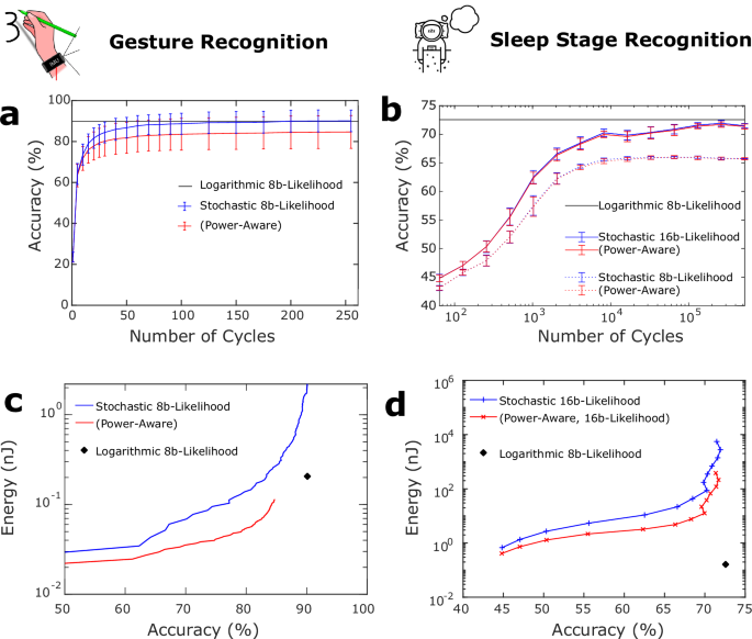
a, b Accuracy of the stochastic machine on a gesture recognition and b sleep stage classification, as a function of number of clock cycles, using the conventional stochastic computing or the power-aware approach. The accuracy of the logarithmic machine (one clock cycle) is plotted as a reference. Error bars are defined in the “Methods” section. c, d Energy consumption as a function of accuracy for c gesture recognition and d sleep stage classification, using the best-performing approaches considered in (a, b). This Figure is obtained by associating several simulation methodologies and shows average results (see the “Methods” section for the details of the energy consumption methodology).

Full size image

From the data displayed in Fig. 5a, we see that stochastic computing, even with just 50 cycles, delivers quality results: 82% accuracy for the conventional strategy and 80% for the power-aware approach. Elevating the cycle count to 255 boosts these figures to 90% and 84%, respectively, while the logarithmic machine consistently achieves 90% accuracy.

When transitioning to the sleep stage classification task, the challenges posed by stochastic computing become more pronounced. As Fig. 5b demonstrates, 8-bit likelihood-based stochastic computing yields a maximum accuracy of 65%, a stark reduction with regard to the 72.6% achieved by the logarithmic approach. Switching to 16-bit likelihoods in stochastic computing does enhance its accuracy to 72%, but requiring a staggering number of clock cycles: 10,000 cycles merely achieve 70% accuracy. Notably, unlike the gesture recognition task, the power-aware approach closely matches the conventional stochastic computing in performance. Note that, as mentioned earlier, the experimental measurements of Fig. 4c use only the last 1000 points of the test dataset, while the simulation studies of Figs. 5 and 6 use the complete test dataset, explaining why the baseline differs slightly from the experiments (see the “Methods” section).

Accuracy of the stochastic (using conventional and power-aware computation) and logarithmic Bayesian machines as a function of the memristor bit error rates for a gesture recognition and b sleep stage classification tasks. This figure is obtained using Monte Carlo simulation (see the “Methods” section). Error bars/shadows represent one standard deviation when repeating the simulation with different memory errors. Stochastic computing simulations in a use 100 cycles, and in b 4096 cycles.

Full size image

The rationale behind these outcomes is intuitive: the sleep stage task inherently deals with low likelihood values, a consequence of its time-dependent characteristics. Specifically, when in a given sleep stage, the likelihood of transitioning to another stage in the succeeding time step, denoted as (pleft(Y(t)={y}_{2}| Y(t-1)={y}_{1}right)), is limited. However, robust EEG and EMG data can counteract these probabilities. This scenario inherently demands the management of low probabilities, a situation where stochastic computing struggles, while logarithmic computing excels. Therefore, the difficulty of managing low probabilities in complex scenarios elucidates why 8-bit likelihood stochastic computing falls short for this task. Furthermore, this complexity explains the high number of clock cycles required by stochastic computing, as well as the comparable performance of power-aware and conventional stochastic computing.

We now extend our comparative analysis to the energy consumption of the machines. To quantify this metric, we employ the evaluation methodology detailed in ref. ⁷, which utilizes industry-standard tools for integrated circuit power assessment, along with value change dump files that represent real tasks (see the “Methods” section). These assessments are based on the 130-nm CMOS process and hafnium oxide memristor technology employed in our test chip.

Figure 5c plots the energy consumption per gesture recognition task as a function of accuracy for both stochastic computing strategies—conventional and power-aware—and the 8-bit likelihood logarithmic machine. The relative energy efficiency of stochastic and logarithmic computation is not obvious in general: a logarithmic consumption necessitates a single clock cycle, but with arithmetic operations (integer addition) that consume much more energy than the simple AND gates used in stochastic computing. The graph reveals that the power-aware approach consistently outperforms the logarithmic machine in terms of energy efficiency. However, it has an accuracy ceiling of 84%, falling short of the 90% accuracy reached by the logarithmic method. On the other hand, conventional stochastic computing only gains an energy advantage for accuracies below 80%, rendering it non-competitive with the logarithmic machine.

In addition to the chip-based evaluations, we benchmarked the energy consumption of the same gesture recognition tasks on a microcontroller unit (MCU), classically used for edge AI applications, and fabricated in a 90-nm CMOS process, similar to the 130-nm used by our machines (see the “Methods” section). The MCU consumed 2.0 μJ per gesture, considerably higher than both the logarithmic and stochastic Bayesian machine.

The results related to the sleep stage classification task, presented in Fig. 5d, indicate a starkly different situation.

Here, the logarithmic approach, with an energy consumption of just 0.15 nJ per cycle, still largely outperforms the MCU, which consumes 1.3 μJ per cycle for the same task (see the “Methods” section). More surprisingly, the logarithmic machine also surpasses both stochastic strategies across all accuracy levels. Although the power-aware method demonstrates notable energy savings over its conventional counterpart—which, at its highest accuracy, consumes even more energy than the MCU—it remains far less competitive than the logarithmic machine. These findings underscore the logarithmic machine’s superior suitability for time-dependent tasks involving low probability values.

Beyond performance and energy efficiency, robustness to memory read errors can be an important challenge in some memristor-based Bayesian machines. Figure 6 presents Monte Carlo simulation results, incorporating artificially induced errors in the memristor arrays (see the “Methods” section). Across both tasks, all strategies display considerable resilience to memory bit error rates, a feature attributable to the very nature of machine learning tasks. Such tasks are generally robust to errors in parameters due to inherent redundancies—for instance, multiple observations can provide overlapping information.

Interestingly, we see in Fig. 6 that the stochastic approaches exhibit heightened resilience with regards to the logarithmic one, but not for the reasons one might initially surmise. Since memory is read once per input presentation, any error is not smoothed out by stochastic computing; instead, it impacts the entire calculation. The greater robustness of the stochastic machines is rather attributable to the linear representation of likelihoods, where bit-flip errors are, on average, less consequential than in a logarithmic representation.

Our results demonstrate that the logarithmic Bayesian machine offers a compelling advantage with regard to stochastic computing, to perform Bayesian inference in scenarios that require handling low-probability values efficiently, such as in the time-dependent task of sleep stage classification. For this task, we saw that logarithmic computation largely beats stochastic computation in terms of latency and energy consumption. Traditional stochastic Bayesian machines have their merits in simpler probabilistic calculations where high accuracy is less critical. We saw that a stochastic machine consumes less energy than the logarithmic design for gesture recognition when an accuracy lower than 84% is targeted.

Stochastic machines are a natural match in a near-memory computing concept, as they use simple arithmetic circuits and involve reduced data movement. We also saw that they are more robust with regard to memory bit errors than the logarithmic design. Still, stochastic machines struggle with precision and latency in cases with low probabilities. The logarithmic approach reduces computational complexity while maintaining accuracy with regard to traditional Bayesian inference by transforming multiplicative operations into simpler integer addition. Therefore, even if it does not match the concept as naturally as the stochastic machine, it still allows using near-memory computation and provides an excellent compromise between the conceptual beauty of stochastic Bayesian machine and non-near-memory-computing approaches.

The logarithmic memristor-based Bayesian machine shows a robust performance across power supply conditions, without the need of any calibration, which we validated experimentally on our prototype integrated circuit. With its proficiency in efficiently handling Bayesian inferences, this machine is particularly suited for edge AI applications.

The proof-of-concept demonstrations in this work, sleep cycle classification, and gesture recognition, highlight the machine’s capabilities, but its true potential lies in addressing high-uncertainty problems with limited data availability. Meaningful applications include scenarios such as medical or structural catastrophe detection, where real-time decision-making is critical despite sparse or incomplete data. Additionally, the machine’s proficiency in handling incomplete datasets from diverse sources opens avenues for applications like sensor fusion in distributed systems. These features position it as a compelling solution for real-world challenges requiring explainable, transparent, and energy-efficient AI.

Future research will focus on scaling the logarithmic Bayesian machine for broader applications and further reducing its power consumption. Integration with other forms of emerging non-volatile memory technologies could also be explored to enhance performance and durability. Moreover, the adaptability of this approach to other types of probabilistic models offers a rich field for further exploration.

Fabrication of the system

The logarithmic Bayesian machine was fabricated using the same flow as the integrated circuits in refs. ^7,34,39. The CMOS part was manufactured by a commercial provider using a low-power 130-nm process that incorporates four metal layers. The memristor arrays consist of a titanium nitride (TiN)/hafnium oxide (HfO_x)/titanium (Ti)/TiN stack. The hafnium oxide layer is 10 nm thick and deposited via atomic layer deposition, with the titanium layer matching this thickness. Memristors have a 300-nm diameter. A fifth metal layer covers the memristor arrays, which are aligned above exposed vias. The input/output pads, designed for a custom probe card, line up along one edge for easier characterization.

Design of the demonstrator

Our system involves 16 memristor arrays embedded directly within the computational architecture (Fig. 2a–d). The design is similar to the one of the stochastic Bayesian machine⁷: while retaining the memory and mixed-signal circuits, we developed an automated design flow using Cadence Innovus, enabling fully automated place-and-route.

The memristor memory arrays are structured as 64-bit cells using a two-transistor, two-memristor (2T2R) configuration, similar to refs. ^7,34 (Fig. 3a). This setup includes thick-oxide transistors that withstand up to five volts, necessary for memristor programming and forming. An important design challenge is the need for three distinct supply voltages:

• VDD (1.2 V nominal) powers the logic and sensing circuits.

• VDDR (up to 5 V) drives the word lines connected to the gate terminals of selection transistors.

• VDDC (up to 5 V) powers the bit lines or source lines of the memory arrays.

Level shifters, located on each row and column of memory arrays, allow converting VDD input signals into VDDR or VDDC voltages (Fig. 3d). These level shifters use thick-oxide transistors and are described in detail in  Supplementary Notes of ref. ⁷. The write circuits and programming strategy of the memristors are identical to the stochastic Bayesian machine and are also described in Supplementary Notes of ref. ⁷. Sensing is performed by precharge sense amplifiers (PCSA)^7,36,37, designed with high-threshold thin-oxide transistors to reduce energy consumption during operations (Fig. 3b). Design and routing of the memristor arrays and their associated mixed-signal circuitry were executed manually using Cadence Virtuoso, and they were simulated with Siemens Eldo.

Digital circuits, such as decoders, adders, and registers, were described in SystemVerilog and synthesized using Cadence Genus and use high-threshold thin-oxide transistors. Placement and routing of the complete design were fully automated using a homemade Tool Command Language (TCL) flow in Cadence Innovus, following a hand-designed floorplan. Physical verifications, including design rule checks, layout versus schematic checks, and antenna effect checks, were conducted using Calibre EDA tools to ensure the integrity and functionality of the final design.

Measurements of the system

Our test procedure is similar to the one used for the stochastic Bayesian machine⁷ (Fig. 4d). Our system is evaluated using a custom-designed 25-pad probe card, which interfaces with a dedicated printed circuit board (PCB) connected via SubMiniature A (SMA) connectors. This PCB links the inputs and outputs of our test chip to an ST Microelectronics STM32F746ZGT6 microcontroller unit, a Keithley triple channel 2230G-30-1 power supply (providing VDD, VDDC, and VDDR), two Keysight B1530A waveform generator/fast measurement units, and a Keysight MSOS204A oscilloscope. The microcontroller is interfaced with a computer through a serial connection, and all other equipment is connected to the computer using a National Instruments GPIB connection. Testing procedures are controlled using a Python script within a Jupyter Notebook, allowing a highly automated testing process.

Before deploying the Bayesian inference capabilities, each memristor undergoes a critical forming operation to establish conductive filaments. This process involves setting VDDC and VDDR to 3.0 volts each, with VDD at 1.2 V. Each memristor is individually addressed by our chip’s digital circuitry, which applies a one-microsecond programming pulse during this operation (see Supplementary Notes of ref. ⁷).

Subsequent to forming, memristors are programmed to either a low-resistance state (LRS) or a high-resistance state (HRS). For LRS programming (SET mode), VDDC is raised to 3.5 V and VDDR to 3.0 V. Conversely, for HRS programming (RESET mode), VDDC is increased to 4.5 V and VDDR to 4.9 V. Programming pulses are applied in opposite polarity to each memristor depending on the desired resistance state (see Supplementary Notes of ref. ⁷).

In SET mode, a 3.0 V gate voltage (VDDR) is applied to the access transistor to control the compliance current, which prevents device damage and ensures robust device endurance. In RESET mode, where compliance is self-regulated due to the memristor’s natural increase in resistance as switching occurs, a 4.9 V gate voltage fully activates the access transistor, minimizing compliance effects. On a separate die designed for fast programming operations, we measured that memristors programmed under these conditions achieve an endurance of approximately one million SET/RESET cycles.

Our memristor configuration employs a two-transistor, two-memristor (2T2R) structure, where data storage is managed through complementary programming: a zero is stored by setting the left memristor (along BL) to HRS and the right (along BLb) also to HRS, while a one is stored by setting the left to LRS and the right to HRS. This complementary scheme enhances the reliability of data storage³⁵. The log-likelihoods used for Bayesian inference are stored as eight-bit integers, as described in the main text.

We employ a program-and-verify scheme: after programming each memristor in a bit cell, we verify the bit using the on-chip precharge sense amplifier. If the programmed state is incorrect, the programming operation is repeated.

Once programmed, the chip no longer requires high voltages. VDD, VDDR, and VVDC are all set to the same supply voltage: by default 1.2 V, and it can be reduced to 0.5 V for power conservation during extended operations. The output from the Bayesian inference processes is captured by the microcontroller and relayed back to the controlling computer for analysis and result compilation.

Definition of the accuracy of the Bayesian machines

To determine the accuracy of the Bayesian machines, we inferred a result y for each element in the test dataset. Each machine employs distinct output evaluation strategies.

For the logarithmic Bayesian machine, the inferred result corresponds to the row with the maximum 8-bit integer output. This selection is straightforward, achieved by taking the argmax over the machine’s outputs in a single cycle.

For the stochastic Bayesian machine, we used two operational modes:

• Conventional mode: In this mode, the machine performs multiple cycles, accumulating bit-stream values across each row to construct a probability distribution. After reaching a pre-defined cycle count, we compute the final output by taking the argmax over this distribution. This approach enhances accuracy through statistical averaging but requires increased latency and energy consumption.

• Power-Aware mode: To minimize energy consumption, this mode employs a cycle-efficient strategy. Instead of averaging over multiple cycles, computation halts as soon as any output row produces a ‘1’ bit, interpreted as the highest probability result. While this early-stopping approach improves energy efficiency, it may slightly compromise accuracy due to its reliance on the initial detected output rather than a fully averaged distribution.

Sleep stage recognition task

We evaluated the performance of the machine using a task focused on sleep stage classification. This task was selected for its representativeness of on-edge computing scenarios, where the energy supply is constrained. Sleep stage classification can provide valuable insights into sleep disorders and overall sleep quality. We employed the DREAMS Subjects Database, consisting of 20 whole-night polysomnography (PSG) recordings from healthy subjects annotated with sleep stages³⁸.

Given the four-input capacity of our logarithmic Bayesian machine test chip, we had to be selective in choosing the types of data to analyze. We opted for the electroencephalography (EEG) and electromyography (EMG) signals, along with prior knowledge of sleep stages. EEG is pivotal for identifying unique brain wave patterns characteristic of different sleep stages, while EMG measures muscle tone, critical for distinguishing rapid eye movement (REM) sleep from other stages.

In the dataset, sleep stages were annotated based on the Rechtschaffen and Kales criteria. We simplified that data into four categories to fit the machine’s capacity of four outputs: awake state, REM sleep, light non-REM sleep (combining American Academy of Sleep Medicine, or AASM, stages 1 and 2), deep non-REM sleep (AASM stage 3).

For model training and testing, we selected the first healthy subject in the DREAMS database. A set of 40 five-second samples for each sleep stage was used for training, while the remaining data served as a test dataset. The restricted training dataset was intentionally chosen to demonstrate the efficacy in a low-data context, which is a distinctive feature of Bayesian approaches^7,10. The experimental measurements of Fig. 4c use only the last 1000 points of the test dataset, while the simulation studies of Figs. 5 and 6 use the complete test dataset.

The design of our Bayesian model was guided by medical knowledge of sleep stages, which have distinctive features in EEG and EMG signals:

• Awake: presence of alpha waves in EEG (8–13 Hz) and high EMG tone;

• REM sleep: low EMG tone;

• Light non-REM sleep: presence of alpha (8–13 Hz) and theta (4–8 Hz) waves in EEG;

• Deep non-REM sleep: presence of delta waves (0.5–4 Hz) in EEG.

Based on this knowledge, and training set accuracy optimization, we chose three observables. Each five-second sample underwent a fast Fourier transform (FFT) for EEG signal analysis, and power spectral density at 1.5 and 9.35 Hz frequencies were designated as the first two observables. The full power of the EMG signal was also computed and used as the third observable. Then, the likelihoods of the Bayesian models for each stage were estimated from the training data, and modeled using a log-normal distribution. The model was then discretized and quantized. Prior probabilities (pleft(Y(t)| Y(t-1)right)) were adjusted based on previous sleep stages to improve the model’s performance. In Fig. 5b, the error bars represent one standard deviation of the mean accuracy of the Bayesian machines when repeating the inference ten times.

Gesture recognition task

The gesture recognition task is taken from ref. ⁷. It is conducted using a dataset collected in our laboratory involving ten subjects. Each subject performed four distinct gestures—writing the digits one, two, three, and a personal signature in the air. The instructions were deliberately vague to encourage natural variation in gesture execution, enhancing the dataset’s diversity. Gestures were captured using the three-axis accelerometer of a standard inertial measurement unit, with each gesture repeated 25–27 times by each subject. The recording duration varied from 1.3 to 3 seconds depending on the subject and the specific gesture. From these recordings, we extracted ten features, encompassing mean acceleration, maximum acceleration across three axes, variance of the acceleration, and both the mean and maximum jerk (rate of change of acceleration). Then we selected the six most useful features (see Supplementary Notes of ref. ⁷).

For training the logarithmic Bayesian machine, we utilized 20 of the 25–27 recordings for each subject, reserving the remaining 5–7 recordings for testing. All reported results use cross-validation with different test/train dataset splits. The training process involved fitting Gaussian distributions to each feature’s data, which was then logarithmically transformed, discretized and quantized to eight bits to suit the logarithmic computing framework. For the stochastic machine, we reproduce the results obtained in ref. ⁷. In Fig. 5a, the error bars represent one standard deviation of the mean accuracy of the Bayesian machines associated with the ten patients.

Analysis of error sources in the logarithmic Bayesian machine

The main paper demonstrates that the accuracy of our logarithmic Bayesian machine decreases when operating at reduced supply voltages (see Fig. 4c). We performed a detailed analysis of the error sources contributing to this behavior. Memristor resistance variability is a key factor affecting the performance of our system. As shown in Fig. 3e, measurements conducted on a separate die with programming conditions equivalent to those used for the test chip reveal this variability. To understand how this variability impacts performance during inference, we conducted SPICE simulations of a memory array column coupled with the PCSA circuit under varying supply voltages. These simulations incorporated Monte Carlo sampling, with 1000 draws for each operating point, to account for the measured variability of the memristors and the global and local variability of the transistors. We studied the proportion of successful reads for supply voltages ranging from 0.7 to 1.2 V at an operating frequency of 10 MHz. Errors begin to appear at a supply voltage below 0.8 V, consistent with the experimental observations in Fig. 3c. At a supply voltage of 0.7 V, the simulated bit error rate is 80%.

The simulations also reveal the origin of these errors. As the supply voltage decreases, the PCSA’s sensitivity to the HRS/LRS resistance ratio increases. When the ratio is low due to reduced HRS resistance, the charge/discharge time of the PCSA remains largely unaffected, and errors are less frequent. However, when the low ratio results from increased LRS resistance, the charge/discharge time is significantly impacted, and the voltage difference between the two branches of the PCSA becomes insufficient for reliable differentiation, leading to reading errors. This behavior is further exacerbated by variability in the properties of the memristor selection transistor and the PCSA transistors, particularly under low supply voltage conditions.

To complement the analysis of errors originating from the memory components, we performed SPICE simulations on the digital circuitry of the chip, focusing on some of the most sensitive circuits of our design, the registers. Our simulations again tested supply voltages ranging from 0.7 to 1.2 V at an operating frequency of 10 MHz. The tests spanned all process corners: As transistor matching is not critical for register functionality, Monte Carlo simulation is not needed. Unlike the analog components, no errors were observed in the digital circuitry under any tested conditions. This confirms that the observed inaccuracies in system performance are primarily attributable to errors in the memristor arrays and the PCSA circuit, rather than the digital components.

Simulation of scaled Bayesian machines

The gesture recognition task requires six inputs with 64 values and, therefore, does not fit on the fabricated Bayesian machines. To evaluate this task, we simulate a scaled-up version of the Bayesian machines, introduced in ref. ⁷ for the stochastic case, which we adapted here to logarithmic computing. The scaled-up machines comprise six columns and four rows of likelihood blocks. These arrays utilize a differential structure similar to our test chip, effectively implementing four kilobits per array. We developed a comprehensive behavioral model of the machines using MathWorks MATLAB to simulate their functional behavior. Additionally, synthesizable SystemVerilog descriptions of the machine were created to allow for digital synthesis and hardware implementation. Test benches were established for both the MATLAB and SystemVerilog models, using consistent input files to ensure thorough testing across all potential inputs and operational cycles. Both models were meticulously verified to ensure they were equivalent under all tested conditions, confirming the accuracy and reliability of our modeling approach. SystemVerilog description of the machines was synthesized and then placed and routed using our chosen semiconductor technology. We conducted post-place-and-route simulations to evaluate the actual performance of the hardware implementation. The results from these simulations were compared with the original MATLAB model. The hardware implementation behaved as expected without any deviations.

Energy consumption estimates

Our energy consumption estimates focus on the inference phase and were obtained using Cadence simulation tools. Experimental energy measurements were not informative, as they are dominated by the capacitance of the outputs in our probe-tested design. Instead, we employed the energy estimation methodology developed in ref. ⁷.

The energy consumption specific to the memristor arrays was calculated using Siemens Eldo circuit simulations. We conducted array-level simulations of the read operation, measuring the energy required to read a single likelihood.

For the digital circuits, energy consumption was assessed using the Cadence Voltus power integrity framework. A typical Bayesian machine operation was simulated with the Cadence ncsim tool, generating a value change dump (VCD) file that captures the dynamic behavior of the device during inference. This VCD file was then used as an input to Cadence Voltus, ensuring that energy estimates accurately represent real-world device operation. Modeling the memristor arrays in Cadence Voltus presented a unique challenge, as memristors are custom components not included in standard foundry libraries. To address this, we developed a MATLAB-based compiler to create a custom liberty file interpretable by Cadence Voltus. This compiler translates the programmed likelihoods within each memory block into a functional description compatible with Cadence Voltus, enabling accurate energy estimates for the memristor arrays during inference. This custom liberty file differs from the one used for the chip design.

The energy estimates for the digital circuits and memristor arrays were then combined to produce the total inference energy consumption values presented in Fig. 5c, d.

Microcontroller unit implementation of Bayesian inference tasks

To evaluate performance in real-world settings, we implemented gesture recognition and sleep cycle classification on an ST Microelectronics STM32F746ZGT6 microcontroller unit (MCU), embedded in a Nucleo-F746ZG development board. This MCU, produced with a 90-nm CMOS process (similar to the 130-nm process used by our Bayesian machine), is a common choice for edge AI tasks. Our implementation was developed in C using the STM32 Cube IDE from ST Microelectronics, with specific optimizations for efficient MCU operation. This implementation uses the same integer logarithmic representation as our logarithmic Bayesian machine and Bayesian inference is performed using eight-bit integer addition.

For each task, the MCU processes all possible inputs sequentially, with an LED blinking every million inferences to enable precise timing measurements. An Ampere meter was used to directly measure the MCU’s energy consumption, isolated from other board components. To determine the energy consumed exclusively for Bayesian inference, we measured a control program performing all operations except the core Bayesian calculations, including input handling and LED blinking. By subtracting the control program’s energy consumption from that of the full task implementation, we obtained an inference-only energy cost of 2.0 μJ per gesture for gesture recognition and 1.3 μJ per measurement for sleep classification.