The physics-based deterministic scenarios for earthquake hazards and losses of the Zhujiangkou fault in southern China

Introduction
The Guangdong-Hong Kong-Macao Greater Bay Area (GGBA), as one of the four major bay areas globally, stands as one of the most modernized and economically vibrant regions in China1. In 2020, the economic output of the GGBA exceeded 1.6 trillion US dollars. This output is comparable to the GDPs of Canada and South Korea, which ranked ninth and tenth globally that year, respectively2. Moreover, the remarkable economic strength of the GGBA has induced a significant siphon effect on population dynamics. In the past decade, the permanent population surged by more than 21 million, reaching approximately 78.01 million in 20203. While the GGBA experiences fewer earthquakes than China’s Sichuan-Yunnan region, it is still considered a seismically active area4,5. Should extreme earthquakes occur, they could profoundly impact the GGBA.
Other major bay areas globally have suffered extensive damage from earthquakes, offering painful lessons and crucial insights. In 1923, the Tokyo Bay Area endured the devastating Mw 7.9 Great Kanto Earthquake, which ignited massive fires, caused numerous building collapses, and triggered floods. This disaster led to over 100,000 fatalities6. The region faced further calamity during the Mw 9.0 Tohoku Earthquake in 2011, significantly damaging its infrastructure, buildings, and economy and resulting in leakage at the Fukushima nuclear plant7. Similarly, the Mw 7.9 San Francisco earthquake in 1906 struck the San Francisco Bay Area, which caused severe damage to the city, including building collapses, widespread fires, and the paralysis of water and transportation systems, resulting in over 3000 fatalities and leaving a large number of residents homeless8. Moreover, the Mw 6.9 Loma Prieta Earthquake in 1989, though of lower magnitude, still caused significant destruction of critical infrastructure such as bridges and highways and disrupted the social functions of urban agglomerations, resulting in 63 deaths, thousands of injuries, and billions in property losses9. These seismic events have driven major bay areas globally to continually improve their earthquake preparedness and mitigation strategies, enhancing their resilience and reducing the impacts of future earthquake disasters.
The Zhujiangkou Fault (ZF) is located in the core region of the GGBA (Fig. 1), surrounded by the most developed large urban agglomerations in China, including Guangzhou, Shenzhen, Hong Kong, and Macau. The fault extends over 90 km and is primarily distributed in the coastal area10. This fault has exhibited a vertical annual slip rate ranging from 0.14 to 0.47 mm/a and presented a main feature of sinistral slip motion since the late Quaternary, indicating a certain seismic potential4,5. Furthermore, the seismicity of the ZF has been further substantiated by combining experimental stress analysis techniques with rock mechanics, assessing the potential maximum magnitude of approximately Mw 7.011. However, due to the historical rarity of earthquakes along the ZF and the scarcity of historical seismic records, there is a lack of scientific seismic design guidelines for the surrounding regions. Moreover, infrastructures, socio-economic systems, and ecological environments are highly vulnerable to extreme seismic events. A destructive earthquake could cause significant and unpredictable impacts on public life, socio-economics, and even national security. Therefore, it is essential to conduct comprehensive research on the ZF and the associated potential earthquake hazards and risks in the GGBA.

The thick red lines illustrate the surface traces of the ZF, whereas the thin orange lines represent the 3D fault plane. The upper side of the 3D body displays the undulating terrain, and the lateral view shows a cross-section of the velocity structure. The top right panel illustrates the study area.
In recent decades, earthquake hazard analysis methods have become critical technologies for reducing earthquake risk. Particularly, empirically-based Ground Motion Prediction Equations (GMPEs) are widely used to estimate ground motion or seismic intensity, often serving as reference standards for seismic-resistant design in engineering projects and land planning12,13. However, the data supporting GMPEs frequently lack records from large earthquakes near faults. This deficiency hampers the ability of GMPEs to accurately interpret the detailed impacts of ground motion near faults, which are often the primary areas of seismic damage14. Furthermore, GMPEs involve an ‘ergodic assumption’, which leads to a lack of precision when predicting ground motion in specific regions based on multi-source data15,16. Failure to effectively consider the ‘spatial correlation’ between adjacent sites often results in underestimating earthquake hazard17,18,19,20. Additionally, existing GMPEs do not adequately address the fault rupture directivity. This limitation results in the inability to fully represent the variability of specific seismic scenarios triggered by different nucleation zones along the same fault.
Physics-based deterministic simulation methods have been validated through recordings at seismic stations and empirical GMPEs21,22. Compared to the traditionally employed empirical GMPEs, these models have shown great potential for accurately assessing earthquake hazards by comprehensively considering the complexities of the source and the multi-physical parameter fields of the subsurface23,24,25,26. Nonetheless, these methods also exhibit certain limitations. Some can calculate only low-frequency ranges, while others employ stochastic methods for high frequencies. Others overlook the impact of complex 3D physical parameters during simulation, such as fault geometry, friction conditions, stress field distribution, rupture directivity, heterogeneous velocity structures, and undulating topography. Alternatively, they utilize kinematic models to characterize the seismic source. Therefore, the results may not be sufficient to fully reflect the potential future earthquake hazards in the target area.
In this study, we have developed physics-based, high-resolution, broadband, deterministic scenarios for earthquake hazards and losses of the Zhujiangkou Fault in the Guangdong-Hong Kong-Macao Greater Bay Area of southern China. This work encompasses most of the crucial elements, from the dynamics of fault rupture, seismic wavefield propagation, and surface ground motion damage to urban agglomeration losses quantitative assessment. The computation considers the actual 3D physical parameter field, including fault geometry structure, focal mechanisms, regional stress fields, fault friction conditions, inhomogeneous velocity mediums, and undulating topography. Specifically, the complex 3D structure of the fault is meshed, and the appropriate earthquake nucleation area is selected through stress analysis. Fault dynamics rupture is calculated using the curved-grid finite difference method to obtain source models capable of characterizing complex source processes of earthquake scenarios. Through the refined strong ground motion simulation, the broadband ground motion distribution has been obtained and validated by the empirical GMPEs. The earthquake loss estimation model based on historical data is used to quantitatively estimate the human and economic losses under different earthquake scenarios. The uncertainty of the results of this study is further discussed through the calculation and analysis of different nucleation depths and topography. The results indicate that the potential earthquake hazards and losses in the northwestern segment of the ZF are significantly higher than those in the southeastern segment. Areas along the Bay in Hong Kong, Shenzhen, Dongguan, and most parts of Macao and Guangzhou face higher earthquake risks.
Additionally, the experimental results highlight the significant impact of dynamics’ rupture directivity on earthquake hazard and loss assessment. For different earthquake scenarios initiated on the same fault within the study area, despite identical input physical conditions and similar fault slip and magnitude, the directivity effect of fault rupture can give rise to vastly different hazards and losses among urban clusters. This study provides important insights for improving the precision of earthquake risk assessments. Moreover, it presents a practical approach for future earthquake disaster prevention efforts, promoting sustainable urban agglomeration development.
Results
Fault dynamic rupture
In this study, ZF is identified as a vertical fault with a main strike of 155°, extending approximately 93 km in length and 10 km in width along the dip (Fig. 2a). To comprehensively assess the potential earthquake hazards along the ZF, six earthquake nucleation zones are set in areas of high shear stress on the fault plane (see Fig. 2e). The curved-grid finite difference method (CG-FDM)27,28 is employed to numerically simulate the dynamic rupture process of the ZF.
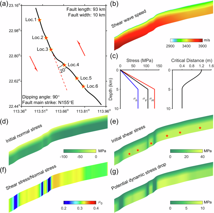
a Surface trace of the ZF. The red arrows denote the movement characteristics of the ZF. The red pentagrams denote the epicenter of the rupture scenarios (at 7.5 km depth). The red dashed line denotes the main strike. b The shear wave velocity distribution on the 3D fault plane. c Depth-dependent fault dynamic rupture simulation parameters. The left column shows the principal stresses and the right column shows the critical slip-weakening distance (Dc). d, e are the resolved initial normal stress (Tn) and initial shear stress (Ts) distribution on the fault plane, respectively. f Distribution of the ratio (μ0) between the initial shear stress and the initial normal stress. g Potential dynamic stress drop defined as Ts – μd·Tn, where μd is the dynamic friction coefficient.
Figure 3 illustrates the results of the dynamic rupture simulation on the ZF, depicting the fault surface slip distribution and isochrones of rupture timing (1 s intervals). Figure 3a–f correspond to Scenarios 1–6, respectively. Scenarios 1–3 are characterized by magnitudes close to Mw 7.0, with Scenario 2 exhibiting the most significant magnitude at Mw 6.92 and a maximum slip displacement of 3.23 m. In contrast, Scenarios 4–6 show significantly lower magnitudes and lateral slip displacements. Scenario 4 features the lowest magnitude at Mw 5.68, and its rupture arrests near the nucleation patch and does not reach the surface. The distribution of subsurface stresses can effectively explain these modes of fault rupture. The ratio of shear stress to normal stress on the fault plane (μ0) appears to be an intuitive measure of the potential rupture capability. Around the source location of Scenario 4, μ0 is notably low (Fig. 2f), severely impedes its rupture propagation outward. The magnitude of stress projected onto the fault plane serves as a mapping expression of the fault geometric structure. In this study, the principal stress direction is N115°, accompanied by a 20° change in strike direction in the central region of the fault. These geometric structures cause variations in the projected values of normal and shear stresses. Ultimately, this leads to the formation of two areas with low μ0 in the middle of the fault plane, making it difficult for earthquakes triggered to rupture along the entire fault completely. Therefore, a bend in the ZF substantially reduces the hazards of triggering extreme earthquake scenarios.
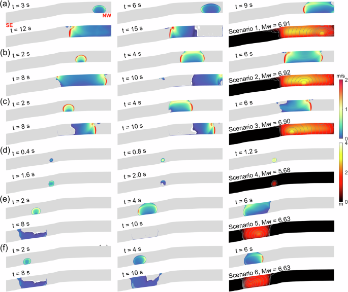
Panels a–f correspond to the six nucleation zones shown in Fig. 2a, named Scenarios 1-6 in this study. Nucleation zones are all located in areas of the fault surface with higher shear stress (Fig. 2e). The first five subfigures in each panel depict the dynamic rupture process. Due to differences in rupture modes, the time intervals between snapshots are set to differ for ease of observation. The last subfigure shows the final slip distribution for each Scenario. The gray solid lines represent isochrones of fault rupture, with time intervals of 1 s.
Overall, the earthquake hazards posed by ruptures initiated on the northern side of the ZF (Scenarios 1–3) are significantly higher than those on the southern side. This disparity leads to a notably increased earthquake risk for Guangzhou compared to other cities within the GGBA. The dynamic rupture processes described herein do not precisely predict actual surface damage, as they are also closely linked to the effects of three-dimensional subsurface medium properties and topography on seismic wave propagation. Consequently, these factors necessitate further calculations and analysis through strong ground motion simulations.
Strong ground motion
We utilize results from dynamic rupture calculations as the input seismic source for strong ground motion simulations. Figure 4a–f show snapshots of seismic wavefields and seismic intensity distributions for Scenarios 1-6, where seismic intensity is derived from the peak ground velocities (PGV) according to the Chinese Seismic Intensity Scale. Overall, the southeastern segment of the ZF exhibits smaller scales of rupture and seismic intensity. Earthquake scenarios originating from the northwestern segment of the fault demonstrate significantly greater potential earthquake hazards than those on the southeastern segment. The seismic intensity maps clearly illustrate that seismic energy is primarily concentrated along the direction of fault rupture propagation. Scenarios 1–3 display markedly different intensity distribution patterns while sharing similar magnitudes and slip distributions (Fig. 3a–c), display markedly different intensity distribution patterns. Similarly, Scenarios 5–6 exhibit the same phenomenon. Scenario 4 features a smaller rupture scale and displays surface energy distribution patterns akin to a double-couple point source.
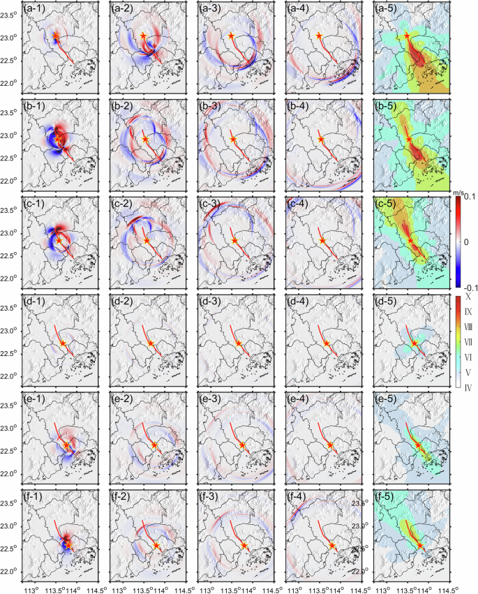
Panels a(1–4) to f(1–4) depict snapshots of seismic wavefields for Scenarios 1-6, respectively. Panels a5–f5 illustrate the seismic intensity distribution for Scenarios 1-6, respectively. Red pentagrams mark the surface projections of the earthquake nucleation zones. Red lines delineate the surface traces of the fault. The base map displays topography and administrative divisions.
The rupture directivity effect is mainly caused by seismic waves emitted early in the rupture, which can interfere constructively with waves emitted later, particularly in the forward direction. The southeast-directed seismic wavefields well demonstrate this in Fig. 4a, b and e, and the northwest-directed wavefields in Fig. 4c, f. The radiated energy from these wavefields aligns closely with the rupture direction, illustrating how rupture directivity strongly correlates with surface energy distribution. In Scenario 1, energy radiation is concentrated in the southeast part of the GGBA, while in Scenario 3, it is focused in the northwest. Scenario 2, which has its nucleation zone in the middle of the northern segment of the fault, shows a more uniform energy distribution along the fault. Similarly, in Scenarios 5 and 6, where the nucleation zones are located at either end of the southeast segment of the fault, the directions of surface energy diffusion are opposite. These observations emphasize the major influence of fault dynamic rupture directivity on the distribution of earthquake hazards and highlight the necessity of incorporating rupture directivity effects in earthquake risk analysis.
Earthquake loss and risk analysis
Based on the Chinese earthquake population and economic loss assessment models29,30, and the spatial distribution of seismic intensity, this study determines the fatality rate and direct economic loss rate for each grid point. By multiplying these loss rates by the population exposure and fixed capital stock exposure at each grid point, the number of fatalities and direct economic losses for that grid point can be calculated. Spatial integration across the entire study area yields the total expected fatalities and economic losses for the entire earthquake scenario. By incorporating the expected loss value and the standard deviation from the loss assessment model into the cumulative normal distribution function, it is possible to evaluate the relative probability of occurrence that the total loss for this earthquake scenario falls within different loss intervals (for detailed process, refer to the Methods section).
Figure 5a–f present the earthquake loss assessment results for earthquake Scenarios 1-6. Each panel displays an assessment of earthquake fatalities on the left and direct economic losses on the right. Pie charts illustrate the quantitative losses for different cities and their percentage of the total loss. The center number in each chart indicates the total loss for that Scenario, and the colors correspond to city coding. Bar charts display the relative probability of the total loss for each Scenario falling within specific loss intervals. The height of the bars indicates the relative probability, with colors transitioning from green (on the left) to red (on the right) to encode the severity of losses. Scenario 1 exhibits the highest potential for earthquake losses, with estimated fatalities exceeding 12,000, and a 57.5% probability that the total fatalities will exceed 10,000. In this Scenario, Shenzhen accounts for the highest proportion of deaths at 47.53%, followed by Guangzhou. Together, these two cities account for over 87% of the total fatalities. The main reason for this phenomenon is that the population of Shenzhen is largely concentrated on the inner side of the Bay Area (many areas have population densities exceeding 20,000 people/km²), which is primarily affected by the seismic high-intensity areas of Scenario 1 (Fig. 4a). Although Guangzhou has a far lower population density in the high-intensity impact areas than Shenzhen, it has a broader affected area and a larger total exposed population. The total economic loss for Scenario 1 is close to RMB 600 billion yuan (1 USD = RMB 7.13 yuan (at 21 August 2024)), with an 82.4% probability that the economic losses will exceed RMB 100 billion yuan. The most probable range for economic losses lies at RMB 100–1000-billion-yuan, accounting for 42.9%. Hong Kong suffers the greatest economic losses, accounting for nearly 40% of the total, contrasting sharply with its share of fatalities (about 6%). This discrepancy is attributed to the extremely high exposure of social assets in highly developed Hong Kong, resulting in a higher percentage of economic loss than fatality in all scenarios.
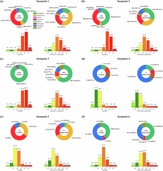
Panels a–f correspond to Scenarios 1–6, respectively. Each panel features estimates of fatalities on the left and economic losses on the right. Pie charts display quantitative loss results for different cities and their respective percentages of the total loss, with the central value representing the total loss for each Scenario. The pie charts employ different colors to represent different cities. Bar charts illustrate the relative probabilities of Scenario total losses occurring within various ranges. The colors of the bars indicate the severity of the losses, progressively intensifying from green to red.
Scenario 4 exhibits the smallest scale of earthquake damage losses (Fig. 5d), with a 96% probability that fatalities will be less than 100% and a 94% probability that economic losses will be under RMB 100 billion yuan. This can be considered a highly probable scenario for minor losses compared to other scenarios. The probability that fatalities will fall within the 1–10 range is the highest, at 47.1%, with an expected value of 9 fatalities. Similarly, economic losses are most likely to fall within the RMB 1–10 billion-yuan range, with a probability of 45.5% and an expected value of RMB 7.2 billion yuan.
Overall, within the same study area, the number of fatalities and economic losses across different earthquake scenarios notably correlate with the magnitude of the earthquakes. For Scenarios 1-3, which have magnitudes ranging from Mw 6.90 to 6.92 (Fig. 3), the probability of fatalities exceeding 1000 people is greater than 92%, and the probability of economic losses exceeding RMB 100 billion yuan is over 78%. However, due to the presence of rupture directivity effects, significant differences in losses still exist between different earthquake scenarios under conditions of the same physical parameters and similar magnitudes. Scenario 2 exhibits the highest magnitude, yet its most likely fatality range is 103–104, comparatively lower than the 104–105 range for Scenarios 1 and 3. However, its anticipated economic loss falls within a moderate range compared to the other two scenarios. These findings indicate that the correlation between earthquake losses and magnitude is not linear, even within the same study area. This highlights the importance of conducting a comprehensive analysis of earthquake hazards and losses considering ground motion and the quantity and value of exposure (population and fixed assets). Furthermore, the variability in exposure across different earthquake scenarios triggered by the same fault is due to the effects of rupture directivity.
This difference is even more pronounced in Scenarios 5 and 6. Despite sharing identical physical parameters and nucleation depths, as well as similar magnitudes, slip distributions, and proximate nucleation locations, the directivity effects of dynamic rupture result in vastly different earthquake losses. The expected fatalities in Scenario 6 are more than three times that in Scenario 5, and the economic losses exceed twice those in Scenario 5. In addition, the interval of fatalities and economic losses corresponding to the potential maximum probability of Scenario 6 is one order of magnitude larger than that of Scenario 5. The spatial variability inherent in these scenarios in the same fault cannot be adequately expressed when calculated for ground motion using traditional empirical GMPEs, with most parameters being identical. Therefore, this study can conduct more accurate and reasonable comprehensive assessments of earthquake risks for specific faults in target study areas by considering the directivity effects of fault rupture.
With its smaller overall population and economic volume, Macao experiences relatively lower loss values than other cities. However, its extremely high population density and exposure to social assets make it highly vulnerable to seismic damage. Therefore, spatial risk analysis of earthquake scenarios along the ZF is necessitated. The analysis in Fig. 6 presents the spatial distribution of earthquake losses and risks for the seven cities bordering the Bay in the GGBA. The six panels correspond to Scenarios 1-6, with the left side of each panel displaying the distribution of risk for earthquake fatalities and the right side depicting the economic losses risk. Based on the loss severity per unit grid area, the earthquake risks are categorized into five levels: very low, low, middle, high, and very high, each represented by color coding. Areas of ‘very high’ risk for earthquake fatalities are primarily concentrated on the eastern to northern sides of the GGBA, particularly near the Bay in Hong Kong, Shenzhen, Dongguan, and most parts of Guangzhou. The Macao Peninsula also falls within the ‘high’ to ‘very high’ risk levels in Scenarios 1-2. Areas of ‘very high’ economic loss risk often correspond to highly urbanized and modernized city areas suffering from high-intensity impacts, specifically near the Bay in Shenzhen, Hong Kong, and Macao. If an earthquake occurs on the northwestern segment of the ZF, most areas of the seven cities near the Bay would be at ‘high’ to ‘very high’ risk levels. Conversely, if an earthquake is nucleated in the southeastern segment, only a few areas would be affected by ‘high’ risks. Overall, future efforts should focus on strengthening earthquake-resistant construction and emergency management levels in the areas from the eastern to northern shores of the Bay. Attention should also be paid to most parts of Guangzhou from the central to southern areas, as regardless of a future earthquake initiated on any segments of the ZF, the proportion of areas in GGBA affected by ‘middle’ or higher risk levels is relatively significant.
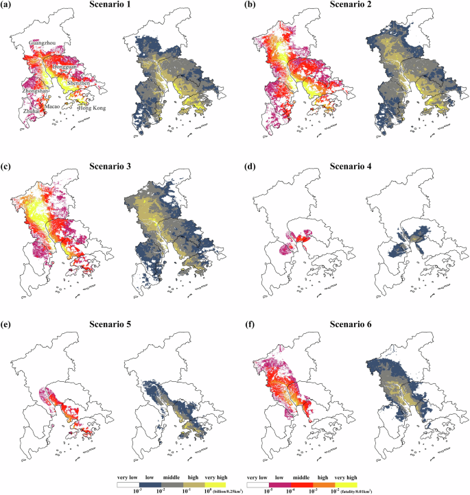
Panels a–f represent Scenarios 1-6, respectively. The left side of each panel shows the fatality risk distribution and the right side shows the economic loss risk distribution. Based on the loss severity per unit grid area, the losses and risks are categorized into five levels: very low, low, middle, high, and very high, each represented by specific color coding.
Discussion
In comparing Scenarios 1-3, it is observable that earthquakes initiated in different nucleation zones along the fault exhibit markedly different patterns of ground motion distribution despite having similar magnitudes. This variation is primarily due to the directivity effects of fault rupture. However, empirically-based GMPEs do not adequately represent these phenomena. To further discuss the advantages of physics-based simulation methods in capturing the directivity of rupture and enhancing the rationality of the present computations, we compared the numerical simulation results of ground motion from Scenarios 1-3 with those predicted by two widely recognized empirical ground motion prediction equations, as depicted in Fig. 7. Grey dots represent the PGV at the surface computational grid points. Blue and red lines represent the predicted PGV and their standard deviations for the BSSA1431 and CB0832 models, respectively. These models employ RJB (the closest distance to the surface projection of the rupture plane) and RRUP (the closest distance to the rupture plane itself) to denote distance. The distances are equal because the fault in this study is a strike-slip fault, and the ruptures occurred at the surface.
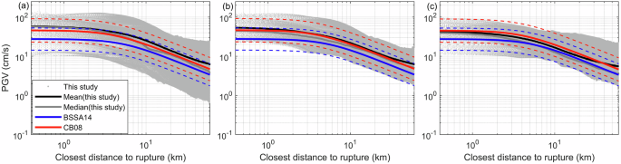
a-c Comparison of the PGV from numerical simulations with the BSSA1431 and CB0832 models for Scenarios 1-3, respectively. Blue and red lines indicate the median values and standard deviations for the BSSA14 and CB08 models. Grey dots represent the PGV at the surface computational grid points, while black and grey solid lines denote the median and mean PGV in this study. Regarding the variations in the discrepancies between this study and GMPEs with distance to rupture, Scenarios 1 and 3 exhibit more significant differences than Scenario 2, which reflects the rupture directivity effects.
Figure 7 shows that the discrepancy between the simulations and the GMPEs increases with the distance from the fault. This trend may be attributed to the physics-based simulations effectively capturing the directivity effects of fault dynamics during rupture. As the propagation distance increases, the impact of rupture directivity becomes more pronounced. Furthermore, the disparity in Scenario 2 is notably less than in Scenarios 1 and 3. This discrepancy may stem from the fact that the epicenter in Scenario 2 is located precisely at the central area of the rupture zone (Fig. 3b), which significantly mitigates the effects of rupture directivity. In Scenario 2, the rupture process occurs symmetrically from both sides of the nucleation zone. The rupture distance at each end is shorter than the unilateral rupture distance observed in Scenarios 1 and 3 (Fig. 3a, c), which means that the impact of rupture directionality is less pronounced. In Scenarios 1 and 3, the nucleation areas are positioned at the edges of the rupture zone, amplifying the rupture directivity effects and increasing the disparity between the numerical simulation results and the GMPEs. Despite these differences, the numerical simulation results and the empirical GMPEs demonstrate good consistency, underscoring the advantages of physics-based simulations in capturing rupture directivity and cross-validating the rationality of the numerical computations.
Using Scenario 2 as a reference, we calculated the earthquake scenario based on the flat topography model, as shown in Fig. 8a. Compared with the flat topography model, the peaks in the western region of Hong Kong show obvious energy concentration in Scenario 2, considering the undulating terrain model. Since the terrain in this study area is relatively flat (Fig. 1), with the highest altitude of about 1 km, the overall difference in the calculated results is very small. The maximum seismic intensity of both scenarios is X, and the calculated PGV means differ by only 3.52%. This study established the nucleation depth at 7.5 km based on the hypocenter depths of small to moderate earthquakes in the surrounding region5. These earthquakes are primarily located within a 5 km to 10 km depth range. Using Scenario 2 as a reference, we calculated additional earthquake scenarios with varying nucleation depths of 5.5 km, 6.5 km, and 8.5 km. The results of the dynamic rupture process are illustrated in Fig. S1. Our findings indicate that the nucleation depth has little impact on the dynamic rupture process in this study area. Consequently, the final slip distribution and the moment magnitude of the fault remain nearly identical across the different nucleation depths. Figure 8b illustrates the seismic intensity distribution for the earthquake scenario with the shallowest nucleation depth of 5.5 km (see Fig. S2 for other scenarios with different nucleation depths). The maximum seismic intensity for all earthquake scenarios is X. The mean PGV values calculated for the two scenarios with nucleation depths of 5.5 km and 7.5 km differ by only 6.7%.
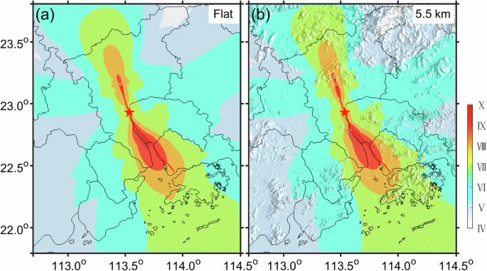
a Seismic intensity distribution for Scenario 2 using a flat topography model. b Seismic intensity distribution for Scenario 2 considering a nucleation depth of 5.5 km.
It is important to note that the ZF has no recorded history of destructive earthquakes, so the results of this study can be viewed as representing potential extreme scenarios of destructive earthquakes along the fault. Some research suggests that the ZF may not be continuous, which could mean that its maximum magnitude might not reach Mw 7.05. Furthermore, our simulations do not account for the viscoelastic attenuation of seismic waves, which could lead to overestimating the earthquake hazards and losses. Other factors that could lead to inaccuracies in assessing earthquake hazards and risks include neglecting the plastic deformation of material responses, failing to incorporate near-surface low-velocity media, and idealizing model setups such as fault geometry, stress configurations, and friction criteria. The onsite geology conditions, such as lithological contacts and geotechnical properties, greatly impact the ground motions and seismic response, especially the shear wave speeds near the ground surface (Vs30). However, we don’t have detailed geology information, such as the detailed velocity model near the ground surface, the soil type or stratification, etc.; it is beyond the scope of this work and our capability. We will discuss the effects of local detailed geological information by cooperating with the relevant department in the future. Additionally, this study provides only a preliminary earthquake risk assessment based on physical simulations, which include ground motion, fatalities, and economic losses. It does not consider more detailed issues such as time exposure, building type, social conditions, etc., which is also the direction of our future work.
This study employs physical-based methods to construct high-resolution, broadband, deterministic scenarios for earthquake hazards and losses of the ZF. It fully considers various factors such as 3D fault geometry structures, stress fields, friction criteria, heterogeneous media, and irregular topography. A comprehensive analysis of earthquake losses and risks in the Guangdong-Hong Kong-Macao Greater Bay Area was conducted. The results indicate that the potential earthquake hazards of the southwestern segment of the ZF are significantly higher than those of the southeastern segment, attributable to the constraints imposed by the fault geometry and stress distribution on its dynamic rupture. Additionally, the study finds that the fault rupture directivity effect, compared to traditionally emphasized factors like site effects and propagation paths, plays a crucial role in determining the distribution patterns of seismic energy on the surface, thereby critically influencing the earthquake hazard analysis.
This study comprehensively assesses potential future earthquake hazards, losses, and risks. The research thoroughly considers the entire physical seismic generation process, from dynamic rupture to ground motion propagation. Compared to traditional methods, this approach enables more realistic and efficient computations. Theoretically, given sufficient computational hardware resources, simulating earthquake wavefields and seismic motions at any bandwidth and spatial resolution is possible. This study offers practical methodologies for regional earthquake prevention and mitigation planning and may provide oppotunities for substantially enhancing urban resilience.
Methods
Fault geometry and nucleation condition
In this study, we construct a 3D nonplanar ZF model based on a study on crustal structure in the Pearl River Delta by the Guangdong Earthquake Agency10. In this model, the fault extends approximately 93 km with a main 155° strike (Fig. 2a). This fault model is set to be vertical, and the fault width along the dip is 10 km according to geological surveys, gravity, and magnetic prospecting results interpretation5,33. Moreover, the fault plane is embedded in an elastic and heterogeneous media model. Figure 2b shows the interpolated shear wave speed distribution on the ZF plane. To initiate the dynamic rupture, we place a circular nucleation patch on the ZF plane, and the radius of the nucleation patch is 2 km. Within the nucleation patch, the initial shear stress is slightly higher (0.5%) than the fault strength. To comprehensively evaluate the earthquake hazards and losses of the ZF, we anchored six nucleation zones (Fig. 2a) according to the regions with large shear stress of the fault, all of which are 7.5 km deep. We used MATLAB R2020b to complete the modeling (fault geometry, stress, velocity medium, etc.).
Initial stresses
We adopt the triaxial stress scheme to configure the initial stress on the fault plane, which consists of three principal compressional stresses, namely, the maximum horizontal principal stress (σH), the minimum horizontal principal stress (σh), and the vertical principal stress (σV). We set σV to be depth-dependent: it increases with depth from 0 to 5 km (σV = 0.8·ρgh, where ρ is the density, g is the gravitational acceleration, and h is the depth) and then remains constant (σV = 0.8·ρg·5000). σH and σh are determined by the relative magnitudes of the three principal stresses. The ratio between these stresses ((σV –σH)/(σh –σH)) in the research area is 0.434. Moreover, the lateral pressure coefficient (σh/σV) is assigned as 0.64 according to the stress states in the upper crust35. Therefore, we have σH = 1.24·σV and σh = 0.64·σV. These depth-dependent principal stresses are schematic in Fig. 2c (left column). The initial normal stress and shear stress are revealed by projecting the triaxial stress onto the fault plane, and the projecting results depend on the angle between the fault strike and the azimuth of the maximum principal stress. The focal mechanisms inverted show that the azimuth of the maximum horizontal principal stress in the research area is approximately N115°5,34. According to this stress scheme, the ZF is characterized by left-lateral strike-slip movement (red arrows in Fig. 2a). By applying the above stress parameters, the resolved normal stress (Tn) and shear stress (Ts) on the ZF are presented in Fig. 2d, e.
Friction parameters
We use the slip-weakening law36 to control the frictional behavior of the ZF during the dynamic rupture simulation, which consists of three key parameters: the static frictional coefficient (μs), the dynamic frictional coefficient (μd), and the critical distance (Dc). The static and dynamic frictional coefficients are 0.4 and 0.24, respectively. These frictional coefficients are obtained by tuning for a maximum moment magnitude of approximately 7. We adopt a depth-dependent critical distance, in which the Dc decreases from 1.2 m at the surface to 0.4 m at a depth greater than 5 km (right column in Fig. 2c). Figure 2f shows the ratio between the shear and the normal stress (μ0) on the ZF, which reveals the fault potential rupture ability. The closer μ0 is to the μs, the easier it is for the rupture to initiate. Moreover, with the friction parameters, we can calculate the potential dynamic stress drop distribution on the fault plane using the initial shear stress minus the residual fault strength (Ts – μd·Tn). The calculated potential dynamic stress drop is presented in Fig. 2g.
CG-FDM
The study utilized the curved-grid finite difference method (CG-FDM)27 to conduct dynamic rupture and strong ground motion simulations. The CG-FDM effectively addresses traction-free boundary conditions in simulations of seismic wave propagation. It employs curved grids to discretize the computational volume and, therefore, can incorporate irregular topography of the simulated research area. The split-node method was introduced to implement the fault boundary conditions and then perform the spontaneous dynamic rupture simulation of the nonplanar faults28. The CG-FDM is distinguished by its computational efficiency and versatility in simulating complex fault geometries, including faults with stepovers and surface roughness. It has been validated against the benchmark problems of the Southern California Earthquake Center-U.S. Geological Survey (SCEC-USGS) dynamic rupture code validation project37. Furthermore, the CG-FDM has been widely validated by simulating the dynamic rupture process of natural earthquakes38,39,40,41 and scenario earthquakes42,43,44.
In fault dynamic rupture simulations, the computational domain is configured in 3D, aligned with the fault strike, normal, and dip directions, with dimensions of approximately 100 km, 20 km, and 14 km, respectively. The grid spacing is set at 50 m, with a time step of 0.004 s over 8000 steps, thus totaling a simulation duration of 32 s. In strong ground motion simulations, the 3D computational domain spans 184 km, 223 km, and 40 km in latitude, longitude, and vertical depth, respectively. The spatial resolution is set at 100 m, resulting in a computational grid scale of 1840 × 2230 × 400. The time step is established at 0.0065 seconds, with a total of 20,000 steps, culminating in a simulation duration of 130 seconds. The calculations fully incorporate the impact of the 3D heterogeneous velocity structure and undulating topography. Topography data are sourced from the Shuttle Radar Topography Mission (SRTM90), with an approximate resolution of 90 m45. Bathymetry data are sourced from the General Bathymetric Chart of the Oceans (GEBCO). We employed a 3D high-resolution crustal shear wave velocity (Vs) model developed by the Guangdong Earthquake Agency, China, based on ambient noise tomography in the Pearl River Delta46. The datasets comprise approximately 30 days of seismic ambient noise recorded by 124 land seismic stations and 28 Ocean Bottom Seismometers (OBS). The minimum shear wave velocity at the surface of the model domain is 2445 m/s, which increases with depth to 4550 m/s. According to the requirements of the CG-FDM for defining the effective wavenumber with six points per wavelength, the upper limit of the effective frequency for ground motion simulation in this study is approximately 4.1 Hz. Figure 1 shows a cross-section of the velocity structure. Figure 2b illustrates the interpolated shear wave speed distribution on the ZF plane.
Earthquake losses estimation
This study utilizes gridded population datasets produced by WorldPop, with a spatial resolution of 100 m47. Provincial fixed capital stock data are calculated using the perpetual inventory method29,30 and are gridded based on nighttime light data48. The research employs the earthquake fatality estimation model49 and the earthquake economic loss estimation model50 based on the development of regression analysis of earthquake disaster loss datasets in China from 1949 to 201951. The following equations are used for estimating fatalities or economic losses:
where ({E}_{F,or,E}) represents fatalities estimated (({E}_{F})) or economic losses estimated (({E}_{E})) for an earthquake. ({r}_{F,or,E}(Int)) represents a fatality or economic loss ratio function based on seismic intensity (Int). The Human Development Index (HDI) is the indicator the United Nations Development Programme proposed for comprehensively evaluating the social development level. (Exposure(gird,event-year,PoporFcs)) represents the current year’s total population (Pop) or fixed capital stock (Fcs) at the grid point within the calculation domain. Φ is the normal cumulative distribution function. ({mathrm{ln}}({E}_{F,or,E})) is the expectation of the distribution, calculated by the loss estimation model with Eq. (1). ζ is the distribution’s standard deviation, representing the uncertainty of the loss estimation model. The reasonableness of the model has been confirmed through normality tests and has been subject to uncertainty analysis49,50.
For the temporal dimension, which encompasses potential impacts on earthquake disaster loss rates due to societal development factors such as building fortification, emergency preparedness, and public awareness, the model adjusts using the HDI. The model employs a zonal strategy to address the differences in seismic structures and economic development that might affect earthquake disaster loss rates in the spatial dimension. This strategy integrates seismological and sociological factors to construct a set of loss rate functions with distinct mathematical expressions for various sub-regions in China. In this study, based on the location of the ZF and the applicable intensity range, Scenarios 1-6 are categorized under the South China fatality assessment model. Scenarios 1-3 fall under the East China economic loss assessment model, while Scenarios 4-6 are grouped under the South China economic loss assessment model. The corresponding standard deviation (ζ) and HDI term coefficients (h) are 1.3539, 1.0; 1.9267, 1.7; and 1.6914, 1.6, respectively36,37. The fatality and economic loss ratio functions are as follows:
Where ({r}_{F}) and ({r}_{E}) represent the fatality ratio and economic loss ratio, respectively. Equation (4) applies to Scenarios 1-3, and Eq. (5) applies to Scenarios 4-6. This approach has been successfully applied to studies of natural earthquakes and setting earthquakes in China in recent years41,44,52,53.


")
Responses