Thermodynamic linear algebra

Basic linear algebra primitives like solving linear systems and inverting matrices are present in many modern algorithms. Such primitives are relevant to a multitude of applications, for example optimal control of dynamic systems and resource allocation. They are also a common subroutine of many artificial intelligence (AI) algorithms, and account for a substantial portion of the time and energy costs in some cases. The most common method to perform these primitives is LU decomposition, whose time-complexity scales as O(d³). Many proposals have been made to accelerate such primitives, for example using iterative methods such as the conjugate gradient method. In the last decade, these primitives have been accelerated by hardware improvements, notably by graphical processing units (GPUs), fueling massive parallelization. However, the scaling of these methods is still a prohibitive factor, and obtaining a good approximate solution to a dense matrix of more than a few tens of thousand dimensions remains challenging.

Exploiting physics to solve mathematical problems is a deep idea, with much focus on solving optimization problems^1,2,3. In the context of linear algebra, much attention has been paid to quantum computers⁴, since the mathematics of discrete-variable quantum mechanics matches that of linear algebra. A quantum algorithm⁵ to solve linear systems has been proposed, which for sparse and well-conditioned matrices scales as (log d). However, the resource requirements⁶ for this algorithm are far beyond current hardware capabilities. More generally building large-scale quantum hardware has remained difficult⁷, and variational quantum algorithms for linear algebra^8,9,10 have battled with vanishing gradient issues^11,12,13.

Therefore, the search for alternative hardware proposals that can exploit physical dynamics to accelerate linear algebra primitives has been ongoing. Notably, memristor crossbar arrays have been of interest for accelerating matrix-vector multiplications^14,15. Solving linear systems has also been the subject of analog computing approaches¹⁶.

Recently, we defined a new class of hardware, built from stochastic, analog building blocks, which is ultimately thermodynamic in nature¹⁷. (See also probabilistic-bit computers^18,19,20 and thermodynamic neural networks^{21,22,23,24,25} for alternative approaches to thermodynamic computing²⁶). AI applications like generative modeling are a natural fit for this thermodynamic hardware, where stochastic fluctuations are exploited to generate novel samples.

In this work, we surprisingly show that the same thermodynamic hardware from Ref. ¹⁷ can also be used to accelerate key primitives in linear algebra. Thermodynamics is not typically associated with linear algebra, and connecting these two fields is therefore non-trivial. Here, we exploit the fact that the mathematics of harmonic oscillator systems is inherently affine (i.e., linear), and hence we can map linear algebraic primitives onto such systems. (See also Ref. ²⁷ for a discussion of harmonic oscillators in the context of quantum computing speedups.) We show that simply by sampling from the thermal equilibrium distribution of coupled harmonic oscillators, one can solve a variety of linear algebra problems.

Specifically we develop thermodynamic algorithms for the following linear algebraic primitives: (i) solving a linear system Ax = b, (ii) estimating a matrix inverse A⁻¹, (iii) solving Lyapunov equations²⁸ of the form (ASigma +Sigma {A}^{top }={mathbb{1}}) and (iv) estimating the determinant of a symmetric positive definite matrix A. We show that if implemented on thermodynamic hardware, these methods scale favorably with problem size compared to digital algorithms. Our numerical simulations corroborate our analytical scaling results and also provide evidence of the fast convergence of these primitives with the wall-clock time, with the speedup relative to digital methods getting more pronounced with increasing dimension and condition number.

We remark that there is a connection between our thermodynamic algorithms and digital Monte-Carlo (MC) algorithms that were developed for linear algebra^{29,30,31,32,33}. Namely, our algorithms can be viewed as a continuous-time version of these digital MC algorithms. However, we emphasize that the continuous time (i.e., physics-based rather than physics-inspired) nature of our algorithms is crucial for obtaining our predicted asymptotic speedup. Additionally, thermodynamic algorithms can be run on a single device³⁴ whereas efficient digital MC linear algebra requires extensive parallelization³⁰.

Algorithmic scaling

In Table 1, we summarize the asymptotic scaling results for our thermodynamic algorithms as compared to the best state-of-the-art (SOTA) digital methods for dense symmetric positive-definite matrices. The derivations of these results can be found in the Supplementary Information (Supplementary Notes 1–5), and are based on bounds obtained for physical thermodynamic quantities, including correlation times, equilibration times, and free energy differences. As one can see from Table 1, an asymptotic speedup is predicted for our thermodynamic algorithms relative to the digital SOTA algorithms. Specifically, a speedup that is linear in d is expected for each of the linear algebraic primitives (ignoring a possible dependence of κ on d). We remark that the complexity of analog algorithms is subtle³⁵ and depends, e.g., on assumptions of how the hardware size grows with problem size. The assumptions made to obtain our scaling results are detailed in the Methods section. In what follows, we systematically present our thermodynamic algorithms for various linear algebraic primitives.

Solving linear systems of equations

The celebrated linear systems problem is to find (xin {{mathbb{R}}}^{d}) such that

given some invertible matrix (Ain {{mathbb{R}}}^{dtimes d}) and nonzero (bin {{mathbb{R}}}^{d}). We may assume without loss of generality that the matrix A in Eq. (1) is symmetric and positive definite (SPD); if A is not SPD, then we may consider the system A^⊤Ax = A^⊤b, whose solution x = A⁻¹b is also the solution of Ax = b. This will affect the total runtime, but still allows for asymptotic scaling improvements with respect to digital methods, in some cases. Also note that constructing an SPD system from a generic one in this way results in the squaring of the condition number, which influences performance. In what follows, we will therefore assume that A is SPD. Now let us connect this problem to thermodynamics. We consider a macroscopic device with d degrees of freedom, described by classical physics. Suppose the device has potential energy function:

where (Ain {text{SPD}}_{d}({mathbb{R}})). Note that this is a quadratic potential that can be physically realized with a system of harmonic oscillators, where the coupling between the oscillators is determined by the matrix A, and the b vector describes a constant force on each individual oscillator. (We remark that while Fig. 1 depicts mechanical oscillators, from a practical perspective, one can build the device from electrical oscillators such as RLC circuits.)

The system of linear equations, or the matrix A, is encoded into the thermodynamic hardware, the system is then allowed to evolve until the stationary distribution has been reached, when the trajectory is then integrated to estimate the sample mean or covariance. This gives estimates of the solution of the linear system or the inverse of A respectively.

Full size image

Suppose that we allow this device to come to thermal equilibrium with its environment, whose inverse temperature is β = 1/k_BT. At thermal equilibrium, the Boltzmann distribution describes the probability for the oscillators to have a given spatial coordinate: (f(x)propto exp (-beta U(x))). Because U(x) is a quadratic form, f(x) corresponds to a multivariate Gaussian distribution. Thus at thermal equilibrium, the spatial coordinate x is a Gaussian random variable

The key observation is that the unique minimum of U(x) occurs where Ax − b = 0, which also corresponds to the unique maximum of f(x). For a Gaussian distribution, the maximum of f(x) is also the first moment 〈x〉. Thus, we have that, at thermal equilibrium, the first moment is the solution to the linear system of equations:

From this analysis, we can construct a simple thermodynamic protocol for solving linear systems, which is depicted in Fig. 1. Namely, the protocol involves realizing the potential in Eq. (2), waiting for the system to come to equilibrium, and then sampling x to estimate the mean 〈x〉 of the distribution. This mean can be approximated using a time-average, defined as

where t₀ must be sufficiently large to allow for equilibration and τ must be sufficiently large for the average to converge to a desired degree of precision. The eventual convergence of this time average to the mean is the content of the ergodic hypothesis^36,37, which is often assumed for quite generic thermodynamic systems. It should be mentioned that the mean could also be approximated as the average of a sequence of samples; however the integration approach has the advantage that it can conveniently be implemented in a completely analog way (for example, using an integrator electrical circuit), which obviates the need for transferring data from the physical device until the end of the protocol.

Figure 2 shows the equilibration process for both a single trajectory (left panel) and the overall distribution (right panel). One can see the ergodic principle illustrated in this figure, since the time dynamics of a single trajectory at thermal equilibrium are representative of the overall ensemble.

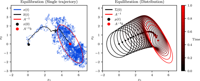
The process of equilibration is depicted on the single-trajectory level (left) and on the distribution level (right). The trajectory dynamics are described by the overdamped Langevin equation and the distributional dynamics by the Fokker-Planck equation⁶⁷. The system displays ergodicity, as the time average of a single trajectory (blue curve, left) approaches the ensemble average (dots, right) in the long-time limit. Time and the coordinate vector (x₁, x₂) are in arbitrary units.

Full size image

The overall protocol can be summarized as follows.

Linear system protocol

• Given a linear system Ax = b, set the potential of the device to

  $$U(x)=frac{1}{2}{x}^{top }Ax-{b}^{top }x$$

  (6)

  at time t = 0.

• Choose equilibration tolerance parameters ({varepsilon }_{mu 0},{varepsilon }_{Sigma 0}in {{mathbb{R}}}^{+}), and choose the equilibration time

  $${t}_{0},geqslant ,{widehat{t}}_{0},$$

  (7)

  where ({widehat{t}}_{0}) is computed from the system’s physical properties or using heuristic methods based on Eqs. (28), (30). Allow the system to evolve under its dynamics until t = t₀, which ensures that (leftVert langle xrangle -{A}^{-1}brightVert /parallel {A}^{-1}bparallel leqslant {varepsilon }_{mu 0}) and (leftVert Sigma -{beta }^{-1}{A}^{-1}rightVert /parallel {beta }^{-1}{A}^{-1}parallel leqslant {varepsilon }_{Sigma 0}).

• Choose error tolerance parameter ε_x and success probability P_ε, and choose the integration time

  $$tau ,geqslant, widehat{tau },$$

  (8)

  where (widehat{tau }) is computed from the system’s physical properties, Eq. (28) or (30). Use an analog integrator to measure the time average

  $${bar{x}}=frac{1}{tau }{int_{{t}_{0}}^{{t}_{0}+tau}}dt,x(t),$$

  (9)

  which satisfies (leftVert Abar{x}-brightVert /parallel bparallel leqslant {varepsilon }_{x}) with probability at least P_δ.

In order to implement the protocol above, the necessary values of ({widehat{t}}_{0}) and (widehat{tau }) must be identified, which requires a more quantitative description of equilibration and ergodicity. To obtain such a description, a model of the system’s microscopic dynamics may be introduced. Given that the system under consideration is composed of harmonic oscillators in contact with a heat bath, it is natural to allow for damping (i.e., energy loss to the bath) and stochastic thermal noise, which always accompanies damping due to the fluctuation-dissipation theorem^38,39. The Langevin equation accounts for these effects, and specifically we consider two common formulations, the overdamped Langevin (ODL) equation and the underdamped Langevin (UDL) equations. In the Methods section, we provide additional details on ODL and UDL dynamics, and we provide explicit formulas for ({widehat{t}}_{0}) and (widehat{tau }) for the overdamped and underdamped regimes.

Estimating the inverse of a matrix

The results of the previous section rely on estimating the mean of x, but make no use of the fluctuations in x at equilibrium. By using the second moments of the equilibrium distribution, we can go beyond solving linear systems. For example it is possible to find the inverse of an SPD matrix A. As mentioned, the stationary distribution of x is ({mathcal{N}}[{A}^{-1}b,{beta }^{-1}{A}^{-1}]), meaning the inverse of A can be obtained by evaluating the covariance matrix of x. This can be accomplished in an entirely analog way, using a combination of analog multipliers and integrators. By setting b = 0 for this protocol, we ensure that 〈x〉 = 0, so the stationary covariance matrix is, by definition

In order to estimate this, we again perform time averages after allowing the system to come to equilibrium

It is therefore necessary to have an analog component which evaluates the product x_i(t)x_j(t) for each pair (i, j), resulting in d² analog multiplier components. Each of these products is then fed into an analog integrator component, which computes one element of the time-averaged covariance matrix

While the equilibration time is the same as for the linear system protocol, the integration time is different, because in general the covariance matrix is slower to converge than the mean. We now give a detailed description of the inverse estimation protocol, assuming ODL dynamics (the corresponding results for underdamped dynamics can be found in Supplementary Note 3). In the Methods section, we provide explicit formulas for ({widehat{t}}_{0}) and (widehat{tau }) for the Inverse Estimation Protocol. We remark that our matrix inversion algorithm is a special case of our general algorithm for solving Lyapunov equations; the latter is presented in Supplementary Note 5.

Inverse estimation protocol

• Given a positive definite matrix A, set the potential of the device to

  $$U(x)=frac{1}{2}{x}^{top }Ax$$

  (13)

  at time t = 0.

• Choose equilibration tolerance parameter ({varepsilon }_{Sigma 0}in {{mathbb{R}}}^{+}), and choose the equilibration time

  $${t}_{0},geqslant ,{widehat{t}}_{0},$$

  (14)

  where ({widehat{t}}_{0}) is computed from the system’s physical properties, Eq. (33) or (34). Allow the system to evolve under its dynamics until t = t₀, which ensures that (leftVert Sigma -{beta }^{-1}{A}^{-1}brightVert /parallel {beta }^{-1}{A}^{-1}parallel leqslant {varepsilon }_{Sigma }).

• Choose error tolerance parameter ε_Σ and success probability P_ε, and choose the integration time

  $$tau ,geqslant, widehat{tau },$$

  (15)

  where (widehat{tau }) is computed from the system’s physical properties, Eq. (33) or (34). Use analog multipliers and integrators to measure the the time averages

  $$overline{{x}_{i}{x}_{j}}=frac{1}{{tau }^{2}}{int_{{t}_{0}}^{tau}}dt,{x}_{i}(t){x}_{j}(t),$$

  (16)

  which satisfies (parallel overline{x{x}^{top }}-{beta }^{-1}{A}^{-1}{parallel }_{F}/parallel {beta }^{-1}{A}^{-1}{parallel }_{F},leqslant ,{varepsilon }_{A}) with probability at least P_ε.

Estimating the determinant of a matrix

The determinant of the covariance matrix appears in the normalization factor of a multivariate normal distribution, whose density function is

and it is therefore natural to wonder whether hardware which is capable of preparing a Gaussian distribution may be used to somehow estimate the determinant of a matrix. This can in fact be done, as the problem is equivalent to the estimation of free energy differences, an important application of stochastic thermodynamics. Recall that the difference in free energy between equilibrium states of potentials U₁ and U₂ is⁴⁰

Suppose the potentials are quadratic, with U₁(x) = x^⊤A₁x and U₂(x) = x^⊤A₂x. Then each integral simplifies to the inverse of a Gaussian normalization factor,

so

This suggests that the determinant of a matrix A₁ can found by comparing the free energies of the equilibrium states with potentials U₁ and U₂ (where A₂ has known determinant), and then computing

Fortunately, the free energy difference ΔF can be found, assuming we have the ability to measure the work which is done on the system as the potential U(x) is changed from U₁ to U₂. According to the Jarzynski equality⁴¹, the free energy difference between the (equilibrium) states in the initial and final potential is

where 〈 ⋅ 〉 denotes an average over all possible trajectories of the system between time t = 0 and time t = τ, weighed by their respective probabilities. This may be approximated by an average over N repeated trials,

However, while Jarzynski’s relation may be applied directly to estimate the free energy difference, this estimator has large bias and is slow to converge. Far more well-behaved estimators have been found based on work measurements. For simplicity, we here provide the expression based on Jarzynski’s estimator, while in the Methods section and in Supplementary Note 4 we refer to more suitable estimators. In summary, the determinant of A₁ is approximated by

In practice we will generally be interested in the log determinant to avoid computational overflow. This is

It is shown in Supplementary Note 4 that to estimate the log determinant to within (absolute) error δ_LD with probability at least P_δ, the total amount of time required is roughly

We also present numerical simulations of a protocol for determinant estimation that does not include directly measuring the work in Supplementary Note 4.

Convergence and comparison to digital algorithms

Convergence

We now present several numerical experiments to corroborate our analytical results. Figure 3A displays the convergence of the absolute error, (| | bar{x}-{A}^{-1}b| |) where ∣∣. ∣∣ denotes the 2-norm, as a function of time for our thermodynamic linear systems algorithm. This plot shows that the expected convergence time to reach a given error is linearly proportional to the dimension of the system, which is in agreement with the analytical bounds that we presented above.

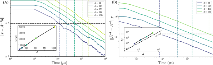
Matrices A are drawn from a Wishart distribution with 2d degrees of freedom. Vertical dashed lines are the times t_C at which error goes below a threshold (horizontal dashed line). Inset: Crossing time t_C as a function of dimension d. A For the linear systems algorithm, a linear relationship between dimension and the analog dynamics runtime is observed. B For the matrix inversion algorithm, a quadratic relationship between dimension and the analog dynamics runtime is observed.

Full size image

Similarly, let us examine the performance of the inverse estimation protocol. We employ the absolute error on the inverse, (parallel {tilde{A}}^{-1}-{A}^{-1}{parallel }_{F}) where ∥ ⋅ ∥_F denotes the Frobenius norm. Figure 3B shows the convergence of the error as a function of the analog dynamics time for our thermodynamic inverse estimation algorithm. We see that the expected convergence time to reach a given error is quadratic (∝ d²) in the dimension, in agreement with the analytical bounds presented above.

Comparison to digital algorithms

Another question of key importance is how the thermodynamic algorithm is expected to perform in practical scenarios, i.e., when being run on real thermodynamic hardware. Due to the hardware being analog in nature, this involves additional digital-to-analog compilation steps. To investigate this question, we consider a timing model for the thermodynamic algorithm, based on the hardware proposal described Ref. ¹⁷ (See Supplementary Note 2 for a brief summary of this hardware, whose dynamics correspond to the overdamped regime as in Eq. (27)). This model includes all the digital, digital-to-analog and analog operations needed to solve the problem, starting with a matrix A stored on a digital device, and sending back the solution x from the thermodynamic system to the digital device. Note that this includes a compilation step that scales as O(d²), which is absent for the digital methods; Cholesky decomposition and the conjugate gradient method are run on a digital computer, and the initial matrix is stored on that same computer, hence there is no transfer cost, unlike for the thermodynamic algorithm. Assumptions about this model are detailed in the Methods section. Note that analog imprecision is not taken into account in these experiments, and is the subject of further investigations⁴².

Figure 4 plots the absolute error for solving linear systems as a function of time for the thermodynamic algorithm (TA), the conjugate gradient (CG) method, and the Cholesky decomposition (which is exact). In panels (A–C) we explore how the methods converge with varying κ and d. While at low dimensions our method performs poorly with respect to the Cholesky decomposition and only slightly better than CG, it becomes very competitive for dimensions d = 1000 and d = 5000. Panels (d) – (f) show the error as a function of time for different condition numbers, at fixed dimension. One can see that as κ grows (as conditioning is worse) our method becomes more competitive with CG. This suggests that, even in practical scenarios where we account for realistic computational overhead issues, our thermodynamic linear systems algorithm can outperform SOTA digital methods, especially for large d and large κ.

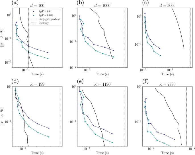
a–c The TA is shown for different values of k_BT (units of 1/γ) for each dimension in {100, 1000, 5000}. Random matrices are drawn from the Wishart distribution and then mixed with the identity such that their condition numbers are respectively 120, 1189, 5995. d–f Same quantities with a fixed condition number κ, respectively 199, 1190, and 7880 for fixed dimension d = 1000. Calculations were performed on an Nvidia RTX 6000 GPU.

Full size image

Figure 4 also shows that the thermodynamic algorithm performs significantly better than the CG method at early times, although the CG method ultimately achieves a higher quality result for later times. This suggests that the thermodynamic algorithm is ideally suited to providing an approximate solution in a short amount of time. Nevertheless, we note that the effective temperature of the thermodynamic hardware is an important parameter, and one can lower this temperature to achieve higher precision solutions from the thermodynamic hardware, as can be seen from the curves in Fig. 4.

Using a timing model similar to that employed for the linear systems protocol, we performed a runtime comparison to Cholesky decomposition for the task of matrix inversion. The results are shown in Fig. 5, where the error is plotted as a function of physical time for dimensions 100, 1000, and 5000. The dashed lines represent the corresponding times for Cholesky decomposition, for given dimensions. We see that as the dimension grows, the advantage with respect to the Cholesky decomposition also grows, thus highlighting a practical thermodynamic advantage. Our method for the inverse estimation therefore has the advantage of having well-defined convergence properties as a function of dimension and condition number (compared to other approximate methods for inverting dense matrices, which do not have well defined convergence properties), as well as leading to reasonable error values in practical settings.

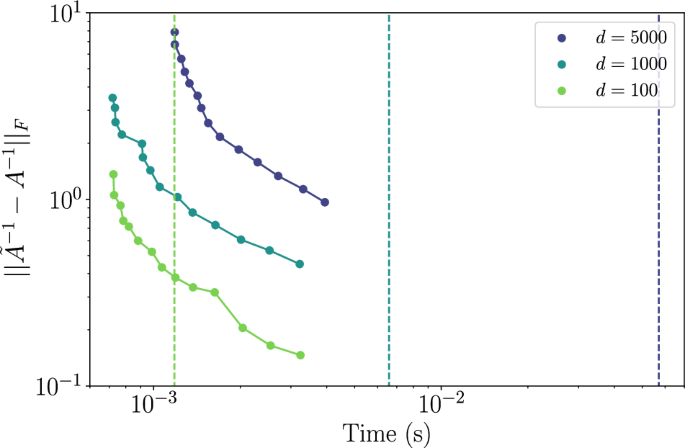
Dimensions d = 100, 1000, 5000, respectively in light green, light blue, and purple, are shown for the thermodynamic algorithm (solid lines) and the Cholesky decomposition (dashed lines). Here the condition numbers are respectively {120, 1189, 5995}. Calculations were performed on an Nvidia RTX A600 GPU.

Full size image

Overall, these numerical experiments highlight the potential utility of thermodynamic hardware by showing the opportunity for speedup over SOTA digital methods, based on a simulated timing model of the thermodynamic device.

Various types of physics-based computers have been devised, which are supposed to expedite calculations by using physical processes to evaluate expensive functions^4,7,43,44,45. These devices (which include quantum computers and a number of distinct analog architectures) have been shown to offer theoretical advantages for solving certain problems, including linear systems of equations, but they have not found common use commercially. A key obstacle to harnessing the power of physical computing is that fluctuations in the system’s state tend to cause errors that compound over time, and which cannot be corrected in a straightforward way⁴⁶ (as can be done for digital computers).

For this reason, we have considered thermodynamic algorithms, which treat the naturally-present fluctuations as a resource, or at the very least are indifferent to them. In fact, we have introduced three distinct classes of thermodynamic algorithms: first-moment based, second-moment based, and all-moment based algorithms. Other thermodynamic algorithms will likely be discovered making use of third and higher moments, implying that such methods form a hierarchy. In some sense, using higher moments allows us to solve “harder” problems, for example inverting a matrix (which uses the second moments) is harder than solving a linear system of equations (which uses the first moment). Whether a precise relationship can be found between computational hardness and the hierarchy of thermodynamic algorithms is currently an open question.

A key property of the system we have studied here that makes it amenable to thermodynamic computing is that the system reaches equilibrium quickly, and the moments of its equilibrium distribution can be efficiently approximated using time averages due to its ergodicity. In extending these methods to other types of dynamics, it is desirable to identify other classes of systems that also equilibrate quickly and for which time averages converge quickly to equilibrium moments. As there is some evidence that this is the case for certain classes of classical chaotic systems as well as quantum systems^47,48, we anticipate that thermodynamic algorithms may be developed in these settings as well.

Another open question concerns the optimality of these new thermodynamic algorithms. Our analysis implies that, while the time and energy costs of linear-algebraic primitives are negotiable, the product of time and energy necessary for a computation is fundamentally constrained (see Methods). It is therefore of interest to search for thermodynamic algorithms which achieve lower values of the energy-time product for these computations, and also to see whether such constraints may apply to other problems as well. We anticipate that non-equilibrium thermodynamics will be a crucial tool in exploring such resource tradeoffs for computation. For example, we have used the fact that a thermodynamic distance may be defined between equilibrium configurations of a system, and this distance determines the minimal amount of dissipated energy necessary to transition from one configuration to another in a finite time^{49,50,51,52,53}; the shorter the time of transition, the more dissipation must occur. Perhaps, then, the search for algorithms which have minimal energy-time product may be framed as a variational problem of minimizing length on the thermodynamic manifold. Although proofs of optimal algorithmic performance are notoriously hard to find in digital computing paradigms⁵⁴, unavoidable resource tradeoffs are relatively mundane in thermodynamic analyses^55,56, suggesting that computational cost may be fruitfully studied within the thermodynamic computing paradigm.

Aside from the theoretical questions mentioned, clearly the task of actually implementing our algorithms remains an important one. Recently, we created an electrical thermodynamic computing device⁵⁷ on a printed circuit board and used it to demonstrate the thermodynamic matrix inversion algorithm presented here, inverting 8 by 8 matrices using 8 coupled electrical oscillators. A potential next step would be to experimentally verify our predicted scaling of integration time with dimension (e.g., linear scaling for linear systems and quadratic scaling for matrix inversion), thus confirming our predicted speedup over digital methods. We anticipate that other researchers may independently seek to verify our results experimentally, leading to a rapid development of thermodynamic hardware. As a result, we predict that these methods will become appealing alternatives to digital algorithms, particularly in settings where it is desirable to trade some accuracy for better time and energy scaling.

In addition to our work’s direct impact, the broader impact is laying the theoretical, mathematical foundations for the emerging paradigm of thermodynamic computing²⁶. Our work provides the first mathematical analysis, as well as the first numerical benchmarks, of potential speedups for thermodynamic hardware. Thus we have taken the somewhat vague notion of thermodynamic computing and made it concrete and precise, with a clear set of applications. Moving forward, we expect new applications to be discovered, beyond linear algebra, since one can simply modify the potential energy function U(x) to solve, e.g., non-linear algebraic problems. There is also the exciting prospect of running multiple applications, such as the linear algebra ones here and the probabilistic AI ones discussed in Ref. ¹⁷, on the same thermodynamic hardware, providing the user with a flexible programming experience. One can envision that much of the amazing technological developments (compilers, simulators, programming languages, etc.) that have happened in quantum computing will likely happen for thermodynamic computing in the near future.

Timing parameters for overdamped and underdamped regimes

Linear systems

For our linear systems algorithm, the overdamped Langevin (ODL) equation takes the form:

where γ > 0 is called the damping constant and β = 1/k_BT is the inverse temperature of the environment. The system has a physical timescale (which is clear from dimensional analysis) that we call the relaxation timeτ_r = γ/∥A∥. The condition number of A is (kappa ={alpha }_{max }/{alpha }_{min }), where α₁…α_d are the eigenvalues of A. With these definitions, we arrive (see Supplementary Note 2 for derivation) at the following formulas for (widehat{{t}_{0}}) and (widehat{tau }) in the overdamped case, which can be used in the linear systems algorithm:

The underdamped model is instead described by the UDL equations,

We define ξ = γ/2M, ({omega }_{j}=sqrt{{alpha }_{j}/M}), and ζ_j = ξ/ω_j. Moreover, a timescale τ_r(UD) can be identified for the underdamped system which is analogous to the quantity τ_r associated with the overdamped system. In particular, we define τ_r(UD) = ξ⁻¹. We introduce a dimensionless quantity χ as well, which is (chi ={(1+xi /{omega }_{min })}^{1/2}{(1-xi /{omega }_{min })}^{-1/2}). With these definitions, we arrive (see Supplementary Note 3 for derivation) at the following formulas for the timing parameters in the underdamped case:

An important distinction between the ODL and UDL regimes is that the random variable x undergoes a Markov stochastic process in the ODL case, but is non-Markovian in the UDL case^58,59. The simple interpretation of this non-Markovianity is that the underdamped system exhibits inertia, which is a form of memory-dependence. This inertia has a non-trivial (and sometimes beneficial) effect on the algorithm’s overall performance, which is apparent from the scaling results in Table 1.

Remark on dependence on the norm of A

Note that the norm ∥A∥ appears in Eq. (28) explicitly in the expression for (hat{tau }) and also enters through the definition of τ_r. We see that ({hat{tau }}_{{rm{r}}}) does not depend on ∥A∥ because the two factors cancel, but ({hat{t}}_{0}) is inversely proportional to ∥A∥. In order to eliminate the dependence on the norm of ∥A∥, we could simply divide A by its norm before applying the algorithm. Then, upon obtaining the solution to the linear system x = A⁻¹b, the vector x would be divided by ∥A∥ to recover the solution to the original problem. However, the computation of ∥A∥ would have a larger polynomial time complexity than our algorithm, so this would eliminate our polynomial speedup. Instead, we can divide A by its largest diagonal element, defining (A{prime} ={a}_{0}A/max {,text{diag},(A)}), where a₀ is a constant with units of γ/t. Now note that

As a lower bound on ∥A∥ gives an upper bound on ({hat{t}}_{0}), we may substitute (parallel A^{prime} parallel) into the above equation for ({hat{t}}_{0}), yielding the following:

The linear system resulting from normalizing A by its largest diagonal element can therefore be solved in linear time. When the solution (x^{prime}) is found, it can then be divided by the largest diagonal element of A to obtain the solution to the original problem. A similar argument applies to Eq. (30) for the underdamped case.

Matrix inversion

The timing parameters for the inverse estimation protocol (as derived in Supplementary Notes 2 and 3) are, for the overdamped case,

and for the underdamped case

Energy-time tradeoff

Note the appearance of the ratio ∥A∥/∥b∥² in the time required to solve a linear system given by Eqs. (28) and (30). It is tempting to imagine that one might solve the system faster simply by multiplying b by some constant c. Then, the time required to solve the system is apparently reduced by a factor of c², and the solution to original problem is obtained (up to a factor of c). A similar approach would be to multiply A by a small number; of course, in practice it is not possible to solve linear systems of equations in vanishingly short periods of time, which is reflected in an energy-time tradeoff. As we explain in Supplementary Note 2, there is an energy cost associated with initializing the system proportional to b^⊤A⁻¹b, and this results in a re-formulation of Eqs. (28) and (30) as lower bounds on the product of energy and time. If ({mathcal{E}}) is the energy required to solve the system Ax = b, and τ is the necessary time, then we have, in the overdamped case:

and in the underdamped case:

This fundamental energy-time tradeoff appears naturally within this computational model. While digital computations can often be accelerated by investing more energy (for example, via parallelization), it is generally less obvious what exact form the relationship between time and energy cost takes, suggesting that thermodynamic algorithms may offer a new and useful perspective on algorithmic complexity.

Detailed algorithmic scaling

In the main text, we presented a simplified version of the detailed table shown in Table 2. Table 2 breaks down the scaling into the overdamped and underdamped regimes, whereas Table 1 just takes the best scalings of our algorithms. The latter is essentially the scaling associated with the underdamped regime. However, in practice, there can be some engineering advantages to working in the overdamped regime, and hence it is useful to see the complexities of both regimes.

Assumptions

A number of assumptions are made in the analytical derivations of the findings presented in the Results section. Certain aspects of the problem have been idealized in order to reveal the fundamental performance characteristics of the thermodynamic algorithms. The main assumptions are the following

• The dynamics of the system may be described by the ODL equation or the UDL equations.

• The potential function U(x), and in particular the matrix A and vector b, can be switched instantaneously between different values.

• The potential energy function U(x) can be implemented to arbitrary accuracy.

• Before a protocol begins, the system may be taken to be in an equilibrium distribution ({mathcal{N}}[0,{beta }^{-1}parallel A{parallel }^{-1}{mathbb{I}}]).

Numerical simulations

We outline the methods used for our numerical simulations of the thermodynamic algorithms. In general, we simulated the overdamped system dynamics because the performance is similar to the underdamped case, and the overdamped system is more numerically stable. The ODL equation, (dx=-{mathcal{A}}x+{mathcal{N}}[0,{mathcal{B}}dt]), is often written using an Itô integral⁶⁰:

where (L{L}^{top }={mathcal{B}}), and in this form it is apparent that the deterministic and stochastic parts of the evolution (the first and second terms above) can be evaluated separately. As this is a Gaussian process, the corresponding Fokker-Planck dynamics are fully captured by the behavior of the first and second moments, which can be evaluated directly using the well-known solution to the Ornstein-Uhlenbeck (OU) process. The JAX⁶¹ library was used to simulate the system at high dimensions, leveraging efficient implementations of matrix exponentials, diagonalization, and convolution to evaluate the various terms in the solution of the OU process. In what follows, we describe the timing model employed for benchmarking our thermodynamic algorithm, assuming an implementation using electrical circuits.

Timing model

To obtain the comparisons to other digital methods, we considered the following procedure to run the TA on electrical hardware. For more details on our model for the hardware implementation we refer the reader to Supplementary Note 2. We take the RC = 1/γ = 1μs, which sets the characteristic timescale of the thermodynamic device. The determinant estimation procedure is excluded here for clarity, as it involves directly measuring work, which may involve a more complicated hardware proposal.

1. 1.

   Compute the values of the resistors ({{R}_{ij},R^{prime}_{i}}) entering the matrix ({mathcal{J}}) that encodes the A matrix.

2. 2.

   Digital-to-analog (DAC) conversion of the ({mathcal{J}}) matrix and the b vector with a given bit-precision.

3. 3.

   Let the dynamics run for t₀ (the equilibration time). Note that for simulations this time was chosen heuristically by exploring convergence in the solutions of the problem of interest.

4. 4.

   Switch on the integrators (and multipliers for the inverse estimation) and let the system evolve for time τ.

5. 5.

   Analog-to-digital (ADC) conversion of the solution outputted from the integrators sent back to the digital device.

For step 1, we measured the time for the digital operation to be performed, and for the other steps we estimated the time, based on the following assumptions:

• 16 bit-precision

• 5000 ADC/DAC channels with a sampling rate: 250 Msamples/s.

• R = 10³ Ω, C = 1 nF, which means RC = 1 μs is the characteristic timescale of the system.

Finally, note that in all cases that were investigated, the dominant contribution to the total runtime was the digital compilation step. This step includes O(d²) operations and involves conversion of the matrix A to ({mathcal{J}}), which is detailed in Supplementary Note 2. Hence some assumptions about the DAC/ADC may be relaxed and the total thermodynamic runtime would be similar. The RC time constant may also be reduced to make the algorithm faster.

Also note that the polynomial complexity of transferring data to and from the thermodynamic computing device should be considered. For the matrix inversion, Lyanpuov equation, and determinant estimation algorithms this does not cause any issue, as the amount of data to be transferred scales with d², which is the same as the time-complexity of the algorithms. For the linear system algorithm, in order to preserve the O(d) time complexity it is necessary for the uploading of the matrix to hardware to be parallelized across O(d) channels, in which case the read/write operations do not affect the polynomial time complexity. An instructive example of a thermodynamic algorithm working as part of a hybrid digital-analog algorithm is presented in Ref. ⁶², where the linear systems algorithm is used as a subroutine in a second-order optimization algorithm.

Noise resilience and error mitigation

To the extent that a circuit can be modeled by equilibrium thermodynamics, and the form and parameters of its Hamiltonian are known, the approach of thermodynamic computing is fully resilient to thermal fluctuations (for example, Johnson-Nyquist noise). However, there are various effects that can cause the continuous-variable Hamiltonian description to be invalid; for example at small currents the discretization of charge leads to significant shot noise which is not accounted for in our formalism. Circuit elements also do not behave in a completely idealized way, for example a capacitor will generally have a capacitance that depends on the applied voltage, leading to a Hamiltonian with higher order terms. Moreover, even if the form of the Hamiltonian is known, the parameters appearing in it cannot be known with certainty, and impedances of circuit components do not exactly match their nominal values, an issue called component mismatch. Finally, even if the electrical components behaved in a completely ideal way and their impedances were known exactly, we may only vary the parameters of a circuit with finite precision; for example, with B bits of precision, we can choose between 2^B possible values for a capacitance in the circuit. Although thermodynamic algorithms offer an appealing resilience to thermal noise, it is necessary to create strategies to mitigate these other sources of error.

In order to address the problems described above, we have begun a comprehensive program of identifying sources of error in thermodynamic computations and finding methods of mitigating these sources of error. Errors caused by imprecision of parameter specification can be significantly reduced using the method proposed in⁴², which is based on stochastically rounding component values between those allowed by the implementation. This method can be used to address imprecision errors, and indeed its experimental implementation resulted in 20% error reduction for matrix inversion⁴². However, it does not help reduce errors caused by component mismatch, so additional strategies are needed. We are presently researching approaches to mitigating component mismatch error, which will be covered in forthcoming work.

Nonlinear behavior of components may prove the most difficult source of error to address, as it involves the form of the Hamiltonian rather than just its parameters, and so cannot be fixed using a simple calibration procedure. To some extent, the degree of nonlinear behavior can be controlled by reducing the amplitude of signals, as nonlinearity typically becomes stronger as the amplitude increases. Unfortunately, reducing the signal amplitude comes with the drawback that a more sensitive measurement device would be needed to obtain the same accuracy. Strategies for reducing error caused by nonlinearities are therefore of great practical importance.