Triangulation for causal loop diagrams: constructing biopsychosocial models using group model building, literature review, and causal discovery

Introduction
In epidemiology and related fields, the adoption of causal diagrams has marked a significant leap forward in drawing causal inferences from observational data. These visual tools synthesize theory-based assumptions about causal relations, enabling the estimation of causal effects for well-defined hypothetical interventions1,2. However, health problems are often complex and characterized by dynamic feedback, adaptation, and interactions across numerous variables at multiple scales of hierarchical organization3,4,5, complicating the search for the underlying network of causality. Consequently, researchers increasingly recommend adopting a multitude of approaches to causality3,4,6 and, in particular, complex systems thinking5,6,7,8.
Among complex systems thinking methods, the causal loop diagram (CLD) is increasingly recognized as a valuable tool in health research9,10. CLDs are causal diagrams that describe hypothesized links between many system variables across relevant space and time scales. A hallmark of CLDs is the inclusion of feedback loops, which are integral to understanding nonlinear changes over time11. Crucially, CLDs provide a conceptual basis for computational system dynamics models that quantify causal relations and can simulate potential ‘what-if’ scenarios10, such as personalized interventions on multiple modifiable risk factors12.
When constructing CLDs, well-established participatory methods, such as group model building (GMB), are commonly used to exploit the collective insights of a diverse group of domain experts13,14. This method of eliciting and synthesizing expert knowledge is particularly beneficial for complex problems where data tend to be scarce and unified causal theories are lacking. However, overreliance on domain experts as a single source of evidence can compromise the reproducibility and structural validity of CLDs15. To mitigate this, researchers increasingly combine multiple approaches, such as GMB and literature review9,10,15. Nevertheless, such approaches may still be prone to subjectivity, relying on the researcher’s or expert group’s assumptions and limitations, which can introduce biases, especially when empirical data are inadequately considered5. Therefore, a mixed-method approach that integrates qualitative and quantitative data is warranted to develop CLDs that more accurately represent real-world systems16.
A promising quantitative approach to identifying causal diagrams from observational data is causal discovery17,18. A famous and classic example is Granger causality19, together with its various refinements (see, e.g., Camps-Valls et al.20 for a brief overview). More recently, initiated by the influential works of Pearl1 and Spirtes, Glymour, and Scheines21, causal discovery has emerged as an established field of research in statistics and machine learning. While the majority of works in this field were primarily intended for cross-sectional data, which captures information at a single point in time, more recent algorithms can efficiently handle longitudinal data, which involves repeated observations of the same subjects over a period of time18,22,23,24. By assessing variables over multiple time points (provided this feedback is not faster than the temporal resolution), dynamic feedback loops can be identified. Although causal discovery does not require a priori domain knowledge of the causal links, its application to real-world data is challenging as causal discovery algorithms can be strongly affected by unmet assumptions regarding, for example, latent confounders, measurement error, selection bias, sample size, and missing data18. Consequently, the resulting causal diagrams might deviate from theory-driven models25 and should be compared to – and validated by – domain knowledge26.
To overcome the individual limitations of causal discovery and GMB, we propose triangulation27 to combine domain expertise from GMB, literature review, and causal discovery (Fig. 1). Triangulation can improve causal inferences by integrating multiple approaches with different and unrelated sources of potential biases4,28,29. For example, in GMB, experts can propose theory-based links not found in the available data. However, the experts may overlook certain links, especially for large systems where considering all possibilities is infeasible10,16 or discipline boundaries do not fully integrate the existing empirical evidence. In contrast, causal discovery provides a data-driven perspective where all possible links are assessed. Thus, it has the potential to identify causal links that experts have overlooked25 or that are not yet established in the scientific literature.

The triangulation of evidence for causal loop diagrams with sources of evidence (domain experts, scientific literature, empirical data) and methods (group model building, literature review, causal discovery).
By triangulating across data sources and methods, causal evidence can, therefore, become increasingly compelling4,27,29. Combining GMB, literature review, and causal discovery in a triangulation approach should enable the accumulation of evidence for specific links between variables, leading to more reproducible and valid causal diagrams while pointing out uncertainties (e.g., if GMB and causal discovery disagree) where further research is needed27.
This paper provides an empirical case example of a mixed methods triangulation approach to CLD development. The case example seeks to map the biopsychosocial feedback mechanisms underlying the course of depressive symptoms in response to a stressor in a healthy adult population. We combine theory-based insights from GMB and literature review with causal discovery using longitudinal data from the Healthy Brain Study30. In this way, we aim to assess how triangulation can impact the development of CLDs.
Results
In this section, we consecutively discuss the case example results from the GMB process, literature review, causal discovery, and their combination through triangulation. Our group of four domain experts included 14 variables in the CLD. These variables came from four domains covered by two experts each: biological, psychological, behavioral, and social. Table 1 provides the baseline characteristics of the measures from the Healthy Brain Study utilized to operationalize the included CLD variables. Supporting evidence for the CLD is provided in the supplementary Excel table and an online interactive version of the CLDs is presented here: https://hbscld.kumu.io/triangulation-for-causal-loop-diagrams.
Group model building
The experts mapped the links between the variables in the GMB sessions. A complete consensus was reached among the expert group regarding each of the 33 links they identified. Figure 2 shows the CLD resulting from these GMB sessions.
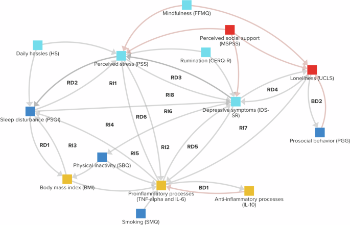
Reinforcing (R) and balancing (B) feedback loops consisting of two (RD, BD) or three variables (RI, BI) have been annotated (see Supplementary Information D for an overview). Grey connections have positive polarity, whereas red connections have negative polarity. The variables’ colors correspond to different dimensions: Social = Red; Behavioral = Dark blue; Psychological = Light blue; Biological = Yellow.
Literature review
After each GMB session, a literature review was conducted for every newly added link. Based on the results of the literature review, the experts adjusted the CLD. The updated CLD is shown in Fig. 3, containing 31 links overall. No literature was found for four of the links. Out of these four, two were removed by the experts (Daily hassles → Sleep disturbance and Proinflammatory cytokines → Perceived stress) because upon further discussion they considered them less plausible. The other two links (Depressive symptoms → Perceived stress and Perceived stress → Sleep disturbance) were kept as the experts still found them plausible with reasonable potential mechanisms of action (dotted arrows, Fig. 3). Nevertheless, these links were considered ‘hypothetical’ due to the lack of literature evidence. Finally, the literature review also sparked a discussion among the experts about the direction of one of the links, leading to the change of Proinflammatory processes → Loneliness into Loneliness → Proinflammatory processes.
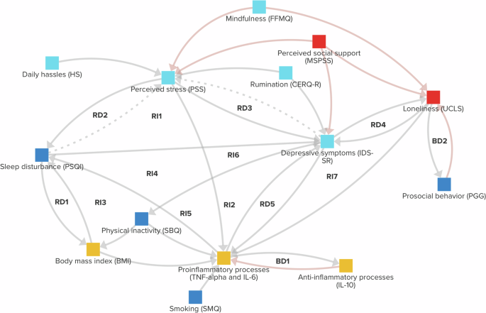
Reinforcing (R) and balancing (B) feedback loops consisting of two (RD, BD) or three variables (RI, BI) have been annotated (see Supplementary Information D for an overview). For dotted links, no supporting literature was found. Grey connections have positive polarity, whereas red connections have negative polarity. The variables’ colors correspond to different dimensions: Social = Red; Behavioral = Dark blue; Psychological = Light blue; Biological = Yellow.
Causal discovery
We then conducted the causal discovery analysis using the J-PCMCI+ algorithm31. The algorithm identified 12 links (Fig. 4 and Table 2) between the variables identified by the experts. We also conducted several sensitivity tests to assess these findings’ robustness. Firstly, we assessed the impact of the significance level of the regression-based conditional independence test, resulting in the same graph with four links missing (Supplementary Information C). Secondly, we assessed the impact of using a different independence test and found the same graph (Supplementary Information C). Finally, to explore the possible impact of selective attrition, we repeated the analysis with only those participants (N = 51) who had complete data at all three assessments (i.e., time points) (Supplementary Information C), where only six out of 11 links corresponded to those found in Table 2. This suggests that causal discovery analysis alone, while informative, may best be complemented with theory-based methods to address data-based limitations.

Straight links correspond to contemporaneous direct causal effects, and curved links correspond to lagged direct causal influences. In our analysis, all lagged links are at lag 1, corresponding to six months. The orange links correspond to a negative effect and the blue links to a positive effect. Lighter colored lines correspond to smaller absolute effects. The algorithm could not orient undirected links (o-o; for example, Daily hassles o-o Perceived stress).
Triangulation
Finally, the experts participated in the final GMB session, combining the information from GMB, literature review, and causal discovery. Figure 5 shows the final CLD resulting from this triangulation process, which contains 36 causal links. An overview of feedback loops is provided in Supplementary Information D.
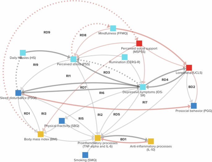
Reinforcing (R) and balancing (B) feedback loops consisting of two (RD, BD) or three variables (RI, BI) have been annotated (see Supplementary Information D for an overview). Bold links are supported by causal discovery. For dotted links, no supporting literature was found. Grey connections have positive polarity, whereas red connections have negative polarity. The variables’ colors correspond to different dimensions: Social Red; Behavioral = Dark blue; Psychological = Light blue; Biological = Yellow.
We distinguished between three possibilities for each link based on the GMB and causal discovery results. (1) Both GMB and causal discovery indicate a link. (2) Causal discovery indicates a link, while GMB does not. (3) GMB indicates a link, while causal discovery does not. The literature review was used to address inconsistencies between the two methods. We took a link as indicated by causal discovery if it had the same polarity as the CLD link and had either the same direction or was undirected (i.e., did not have the opposite direction). Although the ‘o-o’ notation (Table 2) does not indicate a feedback loop, as the method assumes acyclicity for the contemporaneous links, it does not exclude the possibility of a loop in case the assumption of acyclicity is violated. The ‘o-o’ notation could suggest a link in either direction. Therefore, we interpret ‘o-o’ as potential evidence for both links, though it should be noted that this evidence is less strong than that of a directed link.
1) Five links in Table 2 were indicated by both GMB and causal discovery. Each of these links was kept in the CLD by the experts. Four links could not be oriented by J-PCMCI+ (Table 2), so the opposite directions were also considered. This resulted in the addition of Depressive symptoms → Sleep disturbance to the CLD, after which supporting literature was found.
2) Seven links in Table 2 were indicated by causal discovery but not GMB. For these links, the experts either adopted or rejected a link, depending on the presence or absence of scientific literature. One of the links, Anti-inflammatory processes → Proinflammatory processes, was discussed in detail. The experts decided its direction was likely incorrectly identified by J-PCMCI+ and took the link as support for Proinflammatory processes → Anti-inflammatory processes, consistent with the balancing loop (B1) in Figs. 2 and 3. For four of the links, no supporting literature was found (Table 2). One of these links, Loneliness → Perceived social support, was not deemed plausible anymore by the experts and, therefore, not added. Although no literature was found for the other three links, the experts still considered them plausible and added them to the CLD.
3) Most of the links indicated by GMB were not indicated by causal discovery. This discrepancy could arise from data limitations, such as the links not being sufficiently strong within the observed time intervals to be detected. To avoid false negatives, the experts were, therefore, prompted to reevaluate these links only when they were also not supported by the literature review (hypothetical links in Fig. 3). Since the undirected link in Table 2 supported Depressive symptoms → Perceived stress, the discussion was limited to Sleep disturbance → Perceived stress. The experts took into account that, in the causal discovery analysis, Sleep disturbance and Perceived stress were only independent after conditioning on other variables. Out of these variables, Depressive symptoms most strongly diminished the effect. Therefore, the experts considered the indirect pathway Sleep disturbance → Depressive symptoms → Perceived stress more plausible than the direct link, which they removed. The opposite link, Perceived stress → Sleep disturbance was, however, kept since scientific literature was found to support it.
Discussion
In this study, we employed a novel mixed-methods triangulation approach to construct a biopsychosocial CLD, mapping the complex interplay of factors involved in the course of depressive symptoms in response to a stressor in healthy adults. Our CLD provides a preliminary causal mapping of relevant variables, spanning four research domains seldom considered in the same model: biological, psychological, behavioral, and social, relating to our expert group’s fields of expertise. The CLD blends three layers of scientific evidence: consensus from a multi-disciplinary group of domain experts via GMB, knowledge extracted from a literature review, and data-driven detection of causal links through causal discovery using a unique multi-dimensional longitudinal cohort: the Healthy Brain Study30.
While previous studies have compared causal discovery results to expert-based diagrams (e.g., Petersen et al.25), the present study is, to our knowledge, the first to combine causal discovery with GMB, a formal participatory method. Petersen et al.25 found that causal discovery identified links missing from expert-based directed acyclic diagrams that were considered plausible by those same experts. Similarly, in our study, seven links indicated by J-PCMCI+ were not initially indicated by GMB (Table 2), but five of these were incorporated into the final CLD (Fig. 5). This suggests that causal discovery can be particularly beneficial for proposing links that were missed by the experts – who may not fully explore all possible interconnections – or indicate potential research gaps. Furthermore, Petersen et al.25 found large differences between individual expert contributions. Participatory methods like GMB can facilitate greater agreement by actively building consensus through the alignment of mental models32, plausibly leading to higher-quality diagrams. Determining the most effective method for developing causal diagrams, however, requires further empirical exploration through future triangulation studies33.
Based on our case example, we identify three main areas where triangulation positively affects CLD development: comprehensiveness, feedback, and uncertainty. Firstly, by conducting a literature review and causal discovery analysis, the CLD became more comprehensive as several links were added and a few were changed or omitted. Secondly, these changes to the CLD led to modifications in the feedback structure. Feedback loops are critical drivers for the nonlinear behavior of complex systems11, and we found that feedback loops changed between the different steps of the triangulation process. For instance, the reinforcing feedback loop between Perceived stress and Proinflammatory processes (RD6) was removed after the literature review (Fig. 3), and the reinforcing feedback loop between Body mass index and Perceived social support (RD9) was introduced after causal discovery (Fig. 5). Finally, the CLD became more transparent regarding uncertainty, elucidating where experts, literature, and data agreed (i.e., thick and solid lines, Fig. 5), leading to greater confidence, and where they disagreed (i.e., thin or dotted lines). For example, the link Body mass index → Perceived social support might warrant further empirical research, while Perceived stress → Depressive symptoms is more firmly established. This uncertainty regarding causal links can also be incorporated into a computational version of the CLD: a system dynamics model34. Such a model could be used for model comparison with and without hypothetical links, enabling hypothesis testing and a more precise uncertainty quantification10.
Although the CLD was constructed as a proof-of-concept for explorative purposes, it already provides preliminary insights into potential drivers of the course of depressive symptoms over time (the problem behavior; see Fig. 7), such as reinforcing feedback loops35. The CLD reveals short reinforcing feedback loops between Depressive symptoms and Proinflammatory processes (RD5), Perceived stress (RD3), Loneliness (RD4), and Sleep disturbance (RD4) (Fig. 5), illustrating potential self-reinforcing patterns. For example, heightened Perceived stress due to Daily hassles can lead to Depressive symptoms, activating loop RD3. Consequently, Perceived stress and Depressive symptoms can both cause Sleep disturbances, triggering loop RD4, which, in turn, can worsen (the experience of) Daily hassles, forming a longer feedback loop with the shorter loops nested within it (for the sake of clarity, we did not annotate these longer loops in Figs. 2, 3 and 5, see Supplementary Information D). Furthermore, the CLD also describes ‘cross-scale’ loops that involve multiple research domains. For instance, Proinflammatory processes can lead to Loneliness, linking back to Depressive symptoms via loop RD4 and to Proinflammatory processes via loop RI7. We also find biological pathways linking Body Mass Index to Perceived social support (RD9) and Sleep disturbance (RD1), which both impact Prosocial behavior. Interestingly, prosocial behavior is increasingly identified as a major public health asset36, which our CLD suggests can be strongly affected by multiple domains and might help identify intervention strategies to protect an individual’s health.
Limitations of our approach arise from the limitations of the individual methods. Causal discovery is limited by the specific datasets used, which often contain biases arising from, e.g., a significant number of missing values (Table 1), possibly leading to selective loss to follow-up. In our case example, the causal discovery results were indeed sensitive to removing participants with incomplete data from the analysis (Supplementary Information C). This dependency further highlights the need for triangulating across different methods, relying on not only data but also theory. J-PCMCI+ can, in principle, account for unmeasured confounders that are either constant at the subject level or constant over time31. However, we were unable to do so because the Healthy Brain Study includes only three measurements over the span of one year, limiting our ability to correct for context-related confounding beyond sex and education. Additionally, some variables may change at different rates, affecting which links can be found by the algorithm (Table 2). Future studies with longer or more frequent follow-ups may address these issues, though balancing the number of variables with the number of measurements remains challenging. Similarly, the Latent-PCMCI (LPCMCI) algorithm could be considered to account for unmeasured confounding37, but this would also require larger sample sizes to obtain reliable results. On a positive note, our results were robust to changing the independence tests and the method’s hyperparameter settings (Supplementary Information C), and all test statistics’ polarities agreed with the GMB-based CLD link polarities, which adds credibility to the analysis.
Other limitations relate to the literature review. Although a systematic review of scientific literature for all possible links in the CLD would be optimal, this was beyond the scope of our case example and will be infeasible for most research projects (e.g., in our case example, this would have entailed 14 × 13 = 182 separate reviews). In future studies, artificial intelligence tools, e.g., based on natural language processing, might automate some of this work, facilitating a more comprehensive and systematic literature assessment. Considering the above, it should be noted that triangulation is a time-consuming process that introduces complexities in dealing with the different data and conflicting findings. Hence, achieving an optimal balance between efficiency and comprehensiveness is crucial27, depending on the available resources.
Future work could involve alternative approaches to evidence triangulation. For instance, the process could be instantiated with causal discovery instead of GMB, with domain experts interpreting the results and adjusting the diagram according to their domain knowledge, which could then serve as constraints for further causal discovery. Data-driven methods could also be used for variable selection in such an approach. While we focused on triangulation in the mapping phase, triangulation could also enhance the identification of key system variables16. For example, applying explainable machine learning to the Healthy Brain Study data could help identify variables with high predictive accuracy for depressive symptoms. The causal discovery could also be conducted on panel data from multiple studies, and alternative causal discovery methods could also be explored (e.g., TPC23). Lastly, the CLD we developed may be further extended. Future extensions of the CLD could broaden the scope of our case example to encompass more extended time frames and incorporate additional variables that were not yet considered relevant in the demographic of healthy 30-year-olds, such as hippocampal volume.
To conclude, the mixed-methods approach presented in this paper illustrates how evidence triangulation can contribute to constructing more comprehensive CLDs of complex problems with more robust feedback loops and transparency regarding uncertainties in the model’s structure. Our case example combined insights from domain experts, literature, and empirical data, leading to several changes to the CLD during the process and offering a basis for future mental health research. The addition of the literature review and causal discovery helped the experts critically examine their understanding, making the triangulation process recommendable for future studies. As we move forward, the evolution of causal discovery, artificial intelligence, and platforms for interdisciplinary collaborations may help streamline and refine the evidence triangulation process. In turn, this promises to advance our ability to discern the causal networks underlying complex health problems, enabling the development of more valid computational models and intervention strategies with greater effectiveness.
Methods
In CLDs, variables are presented with assumed causal links between them represented as directed arrows. These links can be positive (a change in X gives a change in Y in the same direction) or negative (a change in X gives a change in Y in the opposite direction). Together, the links may form feedback loops. When the number of links with negative polarity is even, these loops are reinforcing, leading to exponential growth or decline. When the number of links with negative polarity is odd, the loops are ‘balancing,’ leading to equilibrium.
Various modeling processes for developing CLDs are documented in the literature11,38,39,40. While these processes may vary in specifics, their fundamental steps are generally comparable. In this project, we employed a CLD development process specifically outlined for health research40. This approach consists of three developmental phases, as depicted in Fig. 6: ‘Define the problem,’ ‘Identify key system variables,’ and ‘Map the system variables.’ In the problem definition phase, we selected a group of domain experts and defined a relevant dynamic problem behavior to model and a model boundary. In the key system variables identification phase, we listed and operationalized an initial set of core variables necessary to explain the problem behavior. Finally, the system variables mapping phase involved connecting the variables in the system to explain the dynamic problem behavior of interest. Since multi-method approaches have already been introduced to address variable selection16, we focus on the triangulation of evidence in the system variables mapping phase. This study was not preregistered.
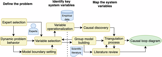
Our approach to developing a causal loop diagram through evidence triangulation from group model building with domain experts, a review of scientific literature, and causal discovery based on empirical data.
Define the problem
Experts selection
Before starting a participatory group modeling process, a multi-disciplinary group of domain experts should first be selected to represent the relevant research domains associated with the research question. The experts should sufficiently cover these domains to promote beneficial debate in the group. In our case example, the expert group for the GMB process was involved in designing the Healthy Brain Study, ensuring the relevance of the measures used to operationalize CLD variables. The Healthy Brain Study is an ongoing project of the Radboud University, the Netherlands, rooted in team science30. The study collected data on a population-based sample comprising 1000 healthy participants aged between 30 and 39. By design, the study seeks to address common limitations in brain research among young adults30 and is, therefore, a good starting point for addressing our research question. In particular, the study takes a holistic approach, providing a wide range of biopsychosocial measures, including cognitive, behavioral, and physiological testing, bio-sampling, questionnaires (e.g., targeting social support and loneliness), and neuroimaging30. Furthermore, the study consists of three assessments (four-month intervals) over one year to gain insight into the within-participant variation of these different measures30, which allows us to address dynamic behavior.
Our specific expert group was formed with the explicit purpose of developing a biopsychosocial health model focused on the longitudinal interplay between social functioning and systemic inflammation on mental health outcomes. The experts, who are all co-authors of this paper, covered the relevant social (MV, JV), behavioral (JV, WFA), psychological (ML, MV), and biological (WFA, ML) research domains.
Dynamic problem behavior
To provide a clear purpose for the GMB process, a relevant “dynamic,” i.e., time-dependent, problem should be defined11,41. Such dynamic problems are commonly visualized using one or multiple reference modes. Reference modes are plots that depict typical problem behavior over time used to illustrate trends, cycles, or patterns in the data, helping researchers identify underlying dynamics and develop hypotheses about the causes of the observed behaviors11,13,39. For instance, if the system moves towards or oscillates around an equilibrium, balancing loops should be included in the CLD40 (e.g., to study concussion42). In our case example, we aimed to map out critical biopsychosocial mechanisms underlying the onset and persistence of depressive symptoms in response to a stressor (e.g., daily hassles). Before starting the GMB process, the experts were involved in two one-hour online brainstorming sessions between March and June 2022, during which the reference mode in Fig. 7 was developed. This reference mode served as a guide for the GMB process. The reference mode shows two hypothetical scenarios. In one scenario, a high frequency and intensity period of daily hassles triggers several reinforcing feedback loops, e.g., involving stress, inflammation, and lifestyle factors. This leads to a rapid increase in depressive symptoms, which are self-limiting but are sustained over time after the daily hassles cease. In the other scenario, a less frequent and intense period of daily hassles also triggers these loops, but to a lesser degree. Consequently, once the daily hassles cease, balancing feedback loops become dominant and return the individual to a normal mood. Given that this reference mode exhibits balancing, equilibrium-seeking behavior, we focused on identifying both potentially balancing and reinforcing mechanisms.

Reference mode involving two hypothetical scenarios where depressive symptoms change over time as a function of a stressor (red).
Model boundary setting
Once the dynamic problem behavior is defined, a model boundary should be established around the problem. The model boundary includes a context of validity with a time frame of interest and the level of aggregation15. In our case example, the expert group also considered the model boundary in the two brainstorming sessions. The boundary was partly driven by the design of the Healthy Brain Study; namely, we assumed a context of healthy 30-year-olds and a total time frame of one year, matching the sample population and follow-up time. Additionally, set a boundary at the individual level, e.g., an individual’s social functioning, but not, e.g., their partner’s. Due to the expertise within our group, we primarily focused on the biological mechanisms related to inflammatory processes.
Identify key system variables
Variable selection
Once the model boundary is established, key variables should be listed that are important for explaining the dynamic problem behavior. A common approach is to involve the GMB experts in selecting the variables11,38,39,40. A standard method for eliciting variables in a GMB process is the nominal group technique43,44, in which the experts individually identify relevant variables and then alternate proposing these variables while arguing for the variable’s relevance.
In our case example, the domain experts individually reviewed relevant scientific literature in their respective domains to identify critical variables. We then applied the nominal group technique during two online sessions of one hour each between June and July 2022. A variable was only included if there was complete consensus by the experts. Although this approach may obscure some uncertainty regarding the CLD, consensus would also be expected to improve the reliability and reproducibility of the CLD, which is beneficial for its integration with causal discovery. JFU was the facilitator during the nominal group technique and GMB sessions. Although the experts could select any variable relevant to the dynamic problem behavior, they primarily focused on variables measured in the Healthy Brain Study. While a CLD should never be limited by measured variables in a specific study, for the case example it made sense to focus on the variables in the Healthy Brain Study, where the data collection was designed for the biopsychosocial context of human brain functioning among young adults30. Nevertheless, for most studies, we recommend conducting GMB first and only then relating the variables to real-world data, as this process might limit the experts to available measures.
Ultimately, a core selection of 20 variables was identified, out of which 14 were ultimately used in the GMB procedure. The experts distinguished between dynamic variables and variables considered static and not yet relevant in the considered age group and time frame (e.g., cognitive functioning, health status, and hippocampal volume). Although incorporating these variables into the CLD was beyond the scope of the present case example, they could be included at a future stage, e.g., when considering adults later in life. Since we focus on young and healthy adults, we assumed these variables do not yet play an important role.
Variable operationalization
A critical step in complementing GMB with causal discovery is operationalizing the CLD variables based on quantitative data. To do this, the experts should consider which measures in the available data best represent the CLD variables. Longitudinal data are ideally used, but cross-sectional data may also suffice, although that will prevent the causal discovery from identifying feedback loops. In our case example, we used panel data (i.e., consisting of multiple individuals over multiple time points) from the Healthy Brain Study resource under release number 2023-1, with cytokine data analyzed by the Radboud Biobank45. For instance, we used experimental behavioral measures to assess prosocial behavior (i.e., the public goods game46), biosamples to assess inflammatory processes, and a validated questionnaire for loneliness47. As the Healthy Brain Study has only recently completed data collection and most of the data is still being analyzed, a specific cohort was defined once 300 participants completed the third and final assessment. By that point, 410 participants had participated in the study, each of whom was incorporated into the cohort. Complete follow-up was available for 73% of individuals and another 4% for the second but not the third assessment. The primary reasons for loss to follow-up were (in order of frequency) the perceived study-related burden, a lack of reachability, and pregnancy or the receipt of a medical diagnosis or treatment.
Not all measures in for the CLD variables were obtained for every participant at every assessment. Various factors contributed to this, including incomplete questionnaires and challenges in obtaining blood samples (e.g., due to concerns about fainting or difficulties in drawing blood samples). Regarding the specific HBS measures of interest, data points were available in the first assessment for 403 participants, with complete data for 189 participants. During the third assessment, 302 participants had measures, of which 98 had complete data. Only 51 participants had complete data across all assessments. Histograms and spaghetti plots are provided for the measures in Supplementary Information B.
Map the system variables
The next phase is to map the hypothesized causal links between the core variables identified during the ‘Identify key system variables’ phase, thereby identifying the dynamic network of causation underlying our problem behavior. In our approach, this phase involves four steps. First, a CLD can be developed with the expert group. Second, the experts review scientific literature for each causal link they identify. Third, empirical data (preferably longitudinal) are used to identify a causal model with causal discovery. Fourthly, these different sources of evidence should be combined into a single causal loop diagram in a triangulation process with the experts. These steps are explained below in further detail and in relation to the case example.
Group model building
GMB is a participatory method for developing systems models, including CLDs. During GMB sessions, a group of expert participants engages in facilitated discussions to align their perspectives and develop a consensus-based model that is more comprehensive than each expert’s mental model. Although CLDs can also be developed from individual expert interviews, GMB produces more comprehensive and coherent CLDs that better explain the system’s dynamic behavior48.
After selecting a core variable list in our case example using the nominal group technique, we conducted seven online GMB sessions with the domain experts between September 2022 and January 2023 to map proposed causal links between the variables. Each session lasted one hour, and at least three out of four experts were present during every session. We also had two additional one-hour discussion meetings where only two experts were present. Between sessions, summary reports were sent to all experts. After each session, the expert who proposed a new link performed a literature review to scrutinize it.
Literature review
Based on the proposed causal links in the GMB, each expert could be asked to conduct a scoping review49 to scrutinize the available evidence for each link belonging to their expertise and provide at least one reference to supporting evidence, if available. During the review, inferring causality from a body of evidence is a nuanced process that lacks a single best prescription4. However, suggested indicators of causality include experimental evidence, temporality (i.e., the exposure preceding the outcome in time), robustness across studies, and plausible intermediary mechanisms consistent with the experts’ knowledge of the system10,50,51. In our case example, the experts conducted reviews after each GMB session for the causal links proposed. Although these reviews were not fully systematic in this explorative project, the experts looked for longitudinal associations that were ideally robust across multiple studies. If no literature supported the link, the group could either remove it if they had lost confidence in it or keep it in the CLD but consider it ‘hypothetical.’
Causal discovery
In parallel to formulating an initial CLD based on expert knowledge and scientific literature, we propose conducting causal discovery whenever sufficient data are available. Ideally, these data are longitudinal, allowing for the identification of time-dependent feedback loops, and comprehensive, like the Healthy Brain Study, where most variables are measured within a single data set so that they can be included in the analysis. Although different types of algorithms exist for causal discovery18, constraint-based algorithms are particularly advantageous due to their flexibility. First, they utilize tests to identify conditional independencies in the data, which can suggest the absence of causal relationships. Moreover, constraint-based algorithms can be applied with a variety of conditional independence tests that are able to deal with different data dependencies (e.g., nonlinearity) as well as data types. In the present study, we had to account for mixed-type data containing both discrete and continuous variables. Second, our study involved multiple time series data sets, and the constraint-based algorithm we utilized (J-PCMCI+, see below) allowed us to handle such instances. We are unaware of a score-based method to deal with multiple time series datasets for mixed-type data. This makes constraint-based algorithms useful for our demands. Moreover, constraint-based causal discovery can be useful even with limited data, as they can exclude certain causal links by detecting these independencies. However, it is important to carefully consider the potential impact of omitted variables, as they can lead to spurious links and incorrect conclusions.
After formulating the initial CLD in our case example, we performed causal discovery on the longitudinal data from the Healthy Brain Study using a simplified version of the J-PCMCI+ algorithm31, which is implemented in the Python package Tigramite version 5.2 (www.github.com/jakobrunge/tigramite). The J-PCMCI+ algorithm is an extension of PCMCI+52, which, in turn, is a time-series adaptation of the widely applied PC algorithm18. Like PC and PCMCI+, J-PCMCI+ is a constraint-based causal discovery algorithm that performs a sequence of statistical independence tests to infer a undirected graph whose (yet undirected) links represent direct causal influences. Then, the algorithm uses the test results and several graphical orientation rules to establish the directionality of these links, that is, to tell apart cause and effect. However, some of the links might remain undirected. Despite its assumption of acyclicity, incorporating time-dependent variables permits the identification of feedback loops within the system, provided these feedback loops do not act on a time scale smaller than the temporal resolution. The algorithm can detect and orient both time-lagged and non-time-lagged (so-called “contemporaneous”) causal links, where the contemporaneous links are assumed to define an acyclic graph and some of the contemporaneous links might remain undirected. Given that the data has only three assessments per individual and that J-PCMCI+ employs a sliding-window approach to generate samples for independence testing, statistically valid tests in JPCMCI+ are possible for, at most, a single time lag. For more details on the algorithm, see Supplementary Information A.
The specific feature of J-PCMCI+ is that it can utilize data from different so-called contexts (here, these are the individual participants) to remove the confounding effect of so-called context variables31. These are variables that are (a) exogenous to the system and (b) constant in time or constant across all contexts (in our case, constant across the participants). In our case example, we included education and sex as context variables. By using a dummy-variables approach, J-PCMCI+ can, in principle, also handle unobserved context variables31. However, in our case example, we did not use this dummy-variables approach for the following reasons: First, to remove the effect of unobserved context-related confounders, a sufficient number of time steps is needed. Since the Healthy Brain Study has only three assessments, this is not the case in our study. Second, time-confounding was deemed unlikely since all measurements were taken within one year. Notwithstanding, the inclusion of education and sex as context variables accounts for at least part of the context-related confounding.
Like all causal discovery algorithms, J-PCMCI+ operates under specific assumptions. For J-PCMCI+, these are the causal Markov and causal faithfulness conditions (see, e.g., Spirtes et al.21 and Peters et al.53), acyclicity of the contemporaneous links (as already mentioned above), stability of the causal structure within the timeframe of the data and across individuals, and the absence of unobserved confounders (except confounders that are constant across time or contexts when dummy variables are used, see above). For independence testing, we used a regression-based independence test for datasets with categorical (i.e., education, sex) and continuous (others) variables with linear dependencies, as implemented in the Tigramite package (RegressionCI). This test is asymptotically equivalent to the test for mixed data suggested in Section 2 of Tsagris et al.54, making the assumption that the respective requirements of the employed regression methods (linear or logistic regression) are met (e.g., independent and homoscedastic Gaussian residuals). However, the regression methods are, to a certain degree, robust against violations of these assumptions54,55. We used a significance level of pcα = 0.05 for the independence tests in the main analysis.
To quantify the strength of the identified links, we then fit linear models of each variable (except context variables) on their parents as estimated with J-PCMCI+ (more details in Runge et al.56). To do this, we assumed that the undirected links (i.e., o-o) had the same direction as in the CLD developed by the domain experts and, in case of a feedback loop, we assessed both directions. Finally, we used the sign of the estimated effects to infer the polarity of the links for the CLD (+ or –).
The J-PCMCI+ algorithm consistently handles missing values for each participant by using only those sliding-window samples with complete data. For instance, say a participant has data for all assessments for some variable ‘(A)’ but only the first assessment for another variable ‘(B).’ Then, when testing for independence of ({A}_{t}) and ({B}_{t}), the algorithm will only draw a single sample from that specific participant (namely, from the first assessment), as opposed to three samples from a second participant who has all assessments for both A and B. Moreover, when testing for independence of ({A}_{t+1}) and ({A}_{t}), the algorithm will draw two samples from both these participants.
Triangulation process
Once all sources of evidence have been collected, we suggest combining them through a triangulation process. In our case example, we adopted the approach that domain experts ultimately decide which links are included to develop a consensus-based diagram10. After obtaining the causal diagram through causal discovery, we thus started a triangulation process with the domain experts to merge it with the expert- and literature-based CLD. We conducted a final two-hour GMB session in September 2023, during which the causal discovery results were discussed with the experts. If an expert considered a link introduced by causal discovery potentially plausible, they were made responsible for the literature review and reported their findings back to the group later.


Responses