Uncovering quantum many-body scars with quantum machine learning

Chaos is a fascinating phenomenon in both classical and quantum systems. In chaotic systems, small perturbations can lead to vastly different dynamical trajectories due to the extreme sensitivity to initial conditions, making long-term predictions highly challenging. The ergodicity and mixing properties of chaotic dynamics underpin the principles of statistical physics and thermodynamics^1,2,3. Occasionally, amidst the chaotic spectrum, there are sometimes integrable, periodic trajectories known as “scars”, where the system temporarily exhibits regular behavior. In contrast, integrable systems are more straightforward to analyze, as their motions are fully predictable and often display periodic dynamics. Besides fully chaotic and integrable dynamics, there exists a class of pseudo-integrable dynamics, where certain chaotic characteristics are present despite some Lyapunov exponents being zero^4,5. These dynamics blend regular and complex behavior, sitting between full integrability and complete chaos.

In quantum many-body systems, chaos reveals itself through the properties of eigenstates, even though the dynamics are governed by the intrinsically linear Schrödinger equation. The eigenstate thermalization hypothesis (ETH)^6,7,8,9,10 assumes that in chaotic systems, the expectation values of local observables appear thermal, even within a single eigenstate. These eigenstates exhibit volume-law scaling of entanglement entropy. When the system evolves from a generic initial state, the phases of the amplitudes on different eigenstates ‘randomize’ rapidly in the unitary evolution, causing the expectation values of local observables to equilibrate to the diagonal ensemble¹¹.

In certain quantum many-body systems, the eigenstate thermalization hypothesis (ETH) can be weakly violated, allowing non-chaotic eigenstates to persist within an otherwise chaotic spectrum. These rare eigenstates, known as quantum many-body scars (QMBSs), represent a vanishing fraction of the entire eigenstates^12,13,14,15. In contrast to chaotic eigenstates, QMBSs offer an intriguing window into non-thermal behavior, posing a challenge for traditional analytical methods. Experimental studies with a 51-atom quantum simulator have observed persistent revivals over long timescales¹⁶, attributed to an evenly spaced tower of QMBSs^12,13. These states are characterized by sub-volume-law entanglement entropy, setting them apart from the typical chaotic eigenstates¹⁷. The strict definition of QMBS remains an open problem, complicated by the complex nature of many-body systems. Identifying atypical eigenstates, which could be candidates for QMBSs, is a challenging task. It is pivotal for understanding ergodicity breaking in quantum systems. Some of these states may be linked to pseudo-integrability due to finite energy and Hilbert space^18,19,20. The weak integrability breaking can exhibit longer thermalization times in quantum many body systems^21,22.

Quantum machine learning (QML) offers powerful tools to study quantum-many-body physics. Among these, quantum convolutional neural networks (QCNNs) are designed to detect patterns in quantum systems and have demonstrated advantages over classical convolutional neural networks when processing classical input data²³. QCNNs have proven particularly effective in classifying different phases of matter in quantum spin systems, as demonstrated both theoretically^24,25 and experimentally²⁶. In particular, QCNNs enable model-independent learning, where the phase boundary can be predicted from synthetic fixed-point states associated with each phase individually²⁷. However, identifying quantum many-body scars (QMBSs) presents a greater challenge than identifying phases due to the scarcity of data, as QMBSs constitute only a vanishingly small fraction of the eigenstates. Recent studies^28,29 have applied unsupervised learning to investigate scars, while ref. ³⁰ has generated scar states by manually engineering conserved quantities. Despite these advances, many other non-thermal states in these systems remain unexplored, highlighting the need for further investigation into hidden eigenstates that could exhibit atypical properties.

We investigate non-thermal states in chaotic systems by resorting to QCNNs. As depicted in Fig. 1, our approach involves training the QCNN on a subset of states within the known subspace of QMBSs. In order to explore the potential of QCNNs in identifying non-thermal states, we investigate three models known to harbor QMBS: xorX model¹⁷, PXP model^31,32 and far-coupling Ising Su-Schrieffer-Heeger(SSH) model³³. In simulations, the QCNN achieves over 99% single-shot measurement accuracy in identifying all known QMBS states. Moreover, it uncovers additional non-thermal states with scar-like properties that extend beyond the established QMBS families. In the xorX model, some of these non-thermal states can be approximately described by spin-wave modes associated with specific quasiparticles. To capture key features of these many-body eigenstates, we develop effective tight-binding Hamiltonians within the quasiparticle subspace. We further validate the QCNN’s performance experimentally on IBM quantum devices. By employing error mitigation techniques, our QCNN achieves a single-shot measurement accuracy of around 63%.

The wave functions inside and outside the scar subspace are treated as two classes that are input to the QCNN as training data. The QCNN consists of convolution layers(C), pooling layers(P) and a fully connected layer(F). Then QCNN is able to identify a larger subspace (dashed circles) of special states that are potential candidates for approximate scars.

Full size image

Models

In this work, we consider three different systems harboring QMBSs, as detailed in this section. Our primary focus is the xorX model. In this model, single spin flip (X) occurs when its nearest neighbors satisfy the exclusive or (xor) condition. The xorX model stands out because it allows for the analytical solution of a family of exact scar states, providing a clear testbed for exploring non-thermal phenomena, though it remains an open question whether other types of scar states exist. The xorX model under open boundary condition (OBC) is described by the Hamiltonian^17,30

where ({sigma }_{i}^{x},{sigma }_{i}^{y},{sigma }_{i}^{z}) are the Pauli-X, Y, Z matrices for the i-th qubit and n is the total number of qubits. In xorX model, the boundary qubits (i = 1, n) are frozen since (left[H,{sigma }_{1}^{z}right]=left[H,{sigma }_{n}^{z}right]=0). We focus on the subspace of (leftlangle {sigma }_{1}^{z}rightrangle =leftlangle {sigma }_{n}^{z}rightrangle =-1). A family of exact scar states in the xorX model can be identified as¹⁷

where ({{mathcal{N}}}_{m}) is the normalization factor and the operator

with projectors ({P}_{i}^{0}={leftvert 0rightrangle }_{i}leftlangle 0rightvert) and ({P}_{i}^{1}={leftvert 1rightrangle }_{i}leftlangle 1rightvert). The domain wall number in the xorX model is conserved as (left[H,{sum }_{i}{sigma }_{i}^{z}{sigma }_{i+1}^{z}right]=0).

The second model we consider in this work is the PXP model, which is derived from the Rydberg atom system in the Rydberg blockade regime³¹. The Hamiltonian of the PXP model is^31,32

where Ω represents the overall energy scale. Notably, the known scar states exhibit a large overlap with the anti-ferromagnetic (Néel) state (| {Z}_{2}left.rightrangle), commonly referred to as Z₂ tower states, which accounts for the persistent oscillations observed in experiments¹⁶. Although a few scar states can be analytically solved using matrix product states³², the nature of other scar states remains an active area of research^22,34,35,36.

The far-coupling Ising SSH model is realized on the platform of superconducting circuit³³. The serpentine routing makes it flexible to tune the coupling between different qubits. The Hamiltonian is

where ({sigma }^{+}=| 1left.rightrangle leftlangle right.0|) and ({sigma }^{-}=| 0left.rightrangle leftlangle right.1|) represent the raising and lowering operators, respectively. J_e and J_o denote the coupling strengths at even and odd positions. J_nn is the next-next-nearest-neighbor coupling strength which breaks integrability. Both numerical simulations and experimental data provide evidence for the existence of scar states in this model, which exhibit a significant overlap with the reference state ({leftvert {Z}_{1001}rightrangle = leftvert 1001rightrangle }^{otimes n/4}).

Non-thermal states

We begin our study with the xorX model in Eq. (1), where there is a family of well-defined exact scar states. Since the exact scar states Eq. (2) are independent of the parameters in the Hamiltonian Eq. (1), the trained QCNN is also parameter independent. Before experimental implementation that will be presented in section Experimental demonstration on quantum device, we first perform numerical simulations on classical computers. After training, the quantum circuit classifies the eigenstates into two types. Interestingly, while the total loss decays during the training, the final converged loss remains near 0.14. Moreover, it successfully recognizes all the exact scar states with an error probability of single-shot measurement less than 1%. This means that the QCNN definitely recognizes all the exact scar state and is expected to do so with sufficient measurement in experiment³⁷. The disparity between the large loss function and the high accuracy in recognizing scar states indicates that the QCNN also classifies some additional states, beyond the known exact scars, as “scar” states. As we detail in section Spin-wave approximation for the marked states in xorX model, we identify a substantial portion of these states as non-thermal states, which bear a significant resemblance to the exact scar states.

The additional non-thermal states have similar energy as the exact scar states, as shown in Fig. 2. These states are situated in the middle of the energy spectrum, distinguishing them from the low-energy integrable modes. Their half-chain entanglement entropy is lower than that of the bulk chaotic states, as shown in Fig. 2a, b, indicating potential deviation from the volume-law entanglement entropy. The QCNN can compensate for deficiencies that the entanglement entropy may fail to distinguish states³⁸. Additionally, the participation ratio (PR), defined as ({sum }_{i}{leftvert langle psi | irangle rightvert }^{4}) for a given state (| psi left.rightrangle) in the computational basis ({| ileft.rightrangle }), is significantly higher than that of the majority of chaotic states, as shown in Fig. 2c, d. They are thus constrained within a smaller Hilbert space compared to chaotic states³⁹.

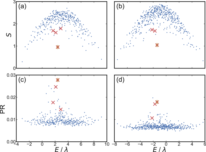
a, c n_dw = 2, b, d n_dw = 3. Other parameters are λ = J = 10Δ. The red crosses are the eigenstates marked by the QCNN. The prisms are the exact scar states. The number of spins is 12 while two of them at the boundaries are fixed.

Full size image

In addition to the static metrics presented above, the existence of scars is often demonstrated through revivals of fidelity in quench dynamics. Here we evolve an initial state under the xorX Hamiltonian in Eq. (1). In Fig. 3, we plot the fidelity of the initial state ({mathcal{F}}={leftvert langle {psi }_{0}| {psi }_{t}rangle rightvert }^{2}) as a function of time, for three different choices of initial states. As expected, an equal superposition of all known exact scar states shows perfect revivals, as illustrated by the blue dashed curve. The superposition of the additional non-thermal states identified by the enhanced QCNN also exhibits revivals, though with a decaying amplitude and not strictly periodic oscillations, as indicated by the red solid curve. In contrast, the superposition of non-marked states does not exhibit any revival (green dashed), as is expected for generic quantum chaotic dynamics. Additional cases of fidelity oscillations are detailed in Supplementary Note 1. Such revivals in the fidelity of initial states highlight a clear distinction between states marked by the QCNN and generic chaotic states, providing further evidence for the non-thermal characteristics of the former.

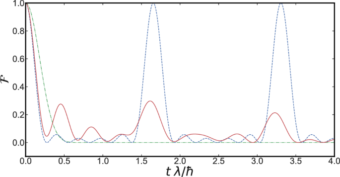
The plot shows fidelity as a function of time, with the initial state being an equal-amplitude superposition of exact scar states (blue dashed line), additional states marked by QCNN (red solid line), and non-marked states (green dash-dotted line). The parameters are the same as in Fig. 2.

Full size image

While the exact scar states of Eq. (2) in the xorX model are parameter independent, we expect that the fraction of these additional non-thermal states can be tuned by varying certain parameters of Hamiltonian (1). For example, upon increasing Δ, pairs of domain walls become more and more confined, which leads to slow thermalization and non-ergodic dynamics⁴⁰. In Fig. 4, we confirm that the ratio of non-thermal states identified by the enhanced QCNN increases with Δ. This further demonstrates the enhanced QCNN’s ability to discern atypical states from the eigenspectrum. On the other hand, when the circuit has more parameters, the criterion becomes stricter. Only states that are close enough to the exact scar states will be marked⁴¹. As a result, the ratio of non-thermal states is smaller, as indicated by the orange dashed line being lower than the blue solid line in Fig. 4.

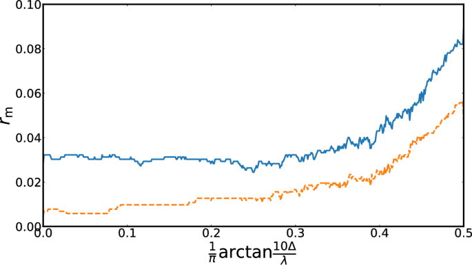
The results are shown for architectures with 2 (blue solid line) and 3 (orange dashed line) convolutional layers before the pooling layers.

Full size image

Spin-wave approximation for the marked states in xorX model

The numerical results presented in the previous section suggest a more detailed study on the nature of the additional non-thermal states found by QCNN in the xorX model in Eq. (1). The PR indicates that these states are predominantly localized within a small subregion of the full Hilbert space. In this section, we demonstrate that some of these non-thermal states can be understood in terms of quasiparticles, specifically magnon bound states. We will construct effective tight-binding Hamiltonians that approximately describe the spin-wave modes of these quasiparticles, reproducing key features of the exact many-body eigenstates.

Integrable states

We begin by considering the simplest scenario. The sequence of exact scar states (| {{mathcal{S}}}_{m}left.rightrangle) in Eq. (2) satisfies m ≤ n/2 for a system of n spins. In particular, the state (| {{mathcal{S}}}_{lfloor n/2rfloor }left.rightrangle) is an anti-ferromagnetic state residing close to the edge of the energy spectrum. For n even, the configuration consistent with the boundary conditions features two domains with different anti-ferromagnetic orders, separated by a single domain wall, as shown in Fig. 5. The Hamiltonian of Eq. (1) acting on this configuration generates a hopping term for the single domain wall and a staggered on-site potential that depends on the sublattice where the domain wall resides. This leads to the following effective single-particle Hamiltonian within the subspace defined by a single domain wall separating two anti-ferromagnetic domains:

where i is the position of the domain wall. In this subspace, the dynamics is fully integrable.

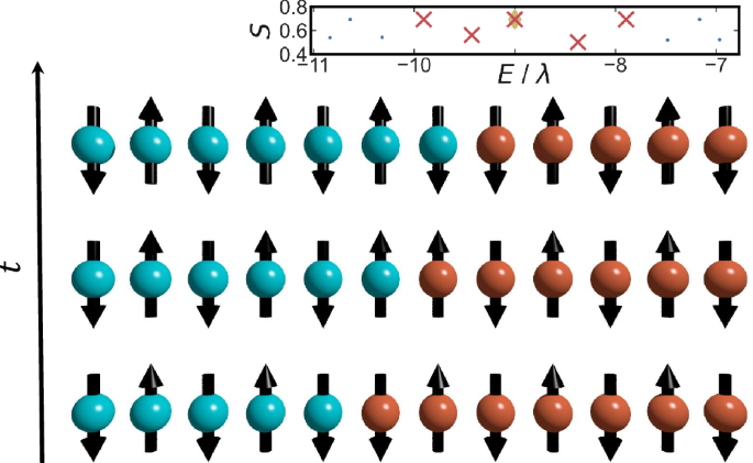
These eigenstates are characterized by distinct eigen-energies with similar entanglement entropy.

Full size image

The above effective Hamiltonian can be readily diagonalized. Under periodic boundary conditions(PBC), the Hamiltonian in momentum space takes the form:

where we have set the lattice spacing to unity. The eigenenergies are ({E}_{k}=pm sqrt{{Delta }^{2}+4{lambda }^{2}{cos }^{2}(k/2)}), with corresponding eigenstates ϕ_k. Under OBC, the eigenstates approximate standing waves, expressed as superpositions of ϕ_k and ϕ_−k. Specifically, these superpositions take the form of (left(|{phi}_{k}rangle+|{phi }_{-k}rangleright)/sqrt{2}) and (left(|{phi }_{k}rangle-|{phi }_{-k}rangleright)/sqrt{2}). These states exhibit low entanglement entropy, characteristic of integrable systems, as shown in the inset of Fig. 5. The QCNN successfully identifies states within this integrable subspace, marking those with energies similar to the exact scar states.

Approximate quasiparticle states

To understand the nature of the states marked as ‘scar like’ by QCNN, we first calculate the mean and variance of their total z-magnetization ({S}_{z}=mathop{sum }nolimits_{i = 2}^{n-1}{sigma }_{i}^{z}), and compare these values with those of typical thermal eigenstates. Figure 6 presents the results for two different domain wall number n_dw sectors. The states marked by QCNN (red crosses) exhibit both a lower average magnetization and a smaller variance compared to typical eigenstates. In the parameter regime with larger Δ, where spin flipping becomes more difficult, the system exhibits increased integrability and better conservation of S_z. Consequently, more eigenstates are marked by QCNN, as shown in Fig. 7.

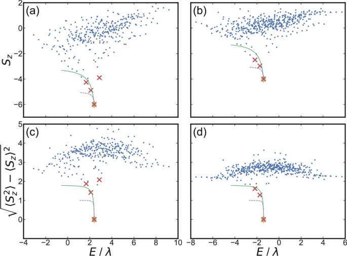
a, c n_dw = 2; b, d n_dw = 3. The red crosses indicate the eigenstates identified by the QCNN. The green solid curves represent analytical results from the ferromagnetic magnon bound state approximation, while the purple dashed curves correspond to those obtained from the anti-ferromagnetic magnon bound state approximation. Other parameters are λ = J = 10Δ.

Full size image

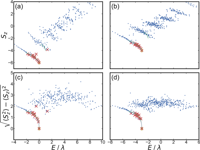
a, c n_dw = 2; b, d n_dw = 3. The red crosses indicate the eigenstates identified by the QCNN. The green solid curves represent analytical results from the ferromagnetic magnon bound state approximation, while the purple dashed curves correspond to those obtained from the anti-ferromagnetic magnon bound state approximation. Other parameters are λ = J = 2Δ.

Full size image

This strongly suggests that these states exhibit a special structure: they can be interpreted as quasiparticles moving within an almost ferromagnetically ordered background (with a negative net magnetization). However, there are two critical differences compared to the quasiparticles in the tower of exact scar states of Eq. (2) and the fully integrable states discussed in the previous section. First, the quasiparticle picture is only approximate. While the exact eigenstates predominantly reside within the quasiparticle subspace, they also have non-negligible components in other configurations within the Hilbert space (see Fig. 9). Second, the quasiparticles in this system are generally more intricate than single magnons or domain walls, often involving longer strings or more complex structures. Moreover, the motion of these quasiparticles typically includes intermediate stages where the size of the quasiparticles first grows and then shrinks (see Fig. 8). In the following, we construct effective Hamiltonians to describe the approximate spin-wave modes of these quasiparticles and demonstrate that they capture similar key features of the exact many-body eigenstates.

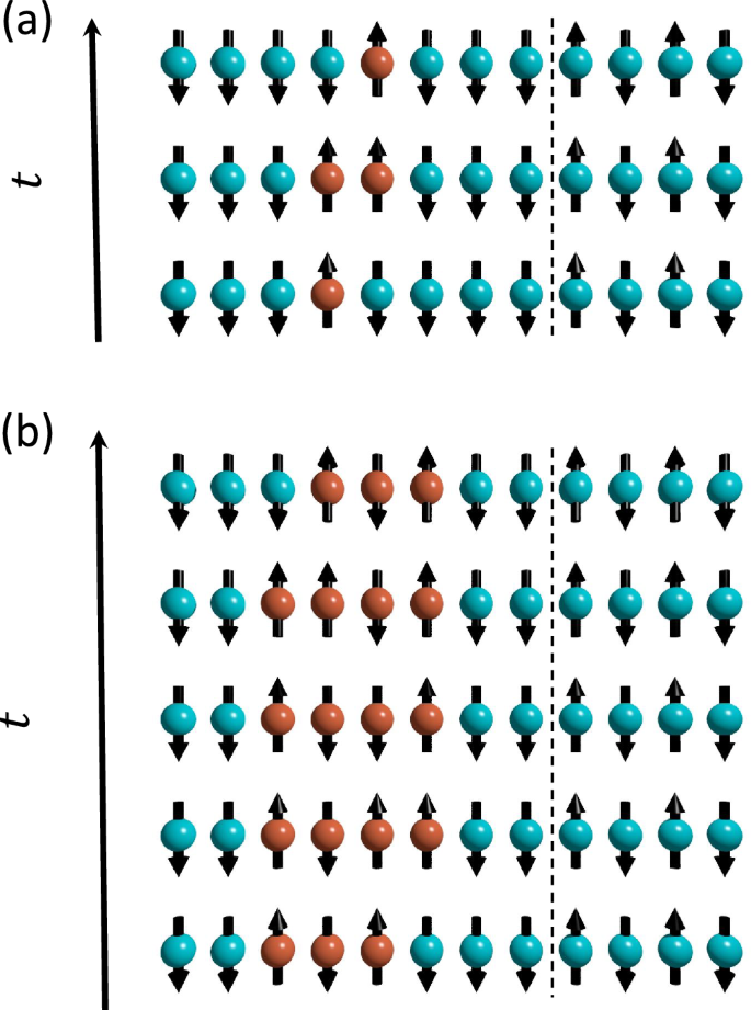
On the left side of the dashed line, blue spins form a ferromagnetic background for the propagation of the bound state. On the right side of the dashed line, blue spins are trapped in an antiferromagnetic configuration. a The motion of a ferromagnetic bound state (red spins). b The motion of an anti-ferromagnetic bound state (red spins).

Full size image

Ferromagnetic magnon bound state

We begin by analyzing the motion of a single magnon in a background of down spins, as depicted in Fig. 8a. In Fig. 9a, b, we present the total weight of each eigenstate within the single-magnon configuration subspace. The data reveal that certain marked states exhibit significantly larger weights in this subspace. The motion of this single magnon will necessarily involve intermediate configurations where the magnon first grows into longer strings and then shrinks. For instance, consider the following intermediate configurations (totaling four configurations): { ⋯ 00111100 ⋯ , ⋯ 0011100 ⋯ , ⋯ 001100 ⋯ , and ⋯ 00100 ⋯ }. The effective Hamiltonian within this subspace has the following form in momentum space (assuming PBC):

The analytical solution of the ground state energy is ({E}_{k}=-Delta sqrt{10+3{u}^{2}+sqrt{64+48{u}^{2}+5{u}^{4}}}/sqrt{2}), where (u=leftvert lambda +lambda {e}^{ik}rightvert /Delta). Under OBC, the system approximately forms standing waves as a superposition of states with momenta ±k. By varying k, we calculate E_k and the corresponding S_z. The relationship between these quantities is illustrated by the green solid curves in Figs. 6 and 7. Most of the marked states closely align with these curves, suggesting that they can indeed be interpreted as spin-wave modes. Furthermore, as Δ increases, the agreement between the marked states and the analytical approximation improves, as shown in Fig. 7.

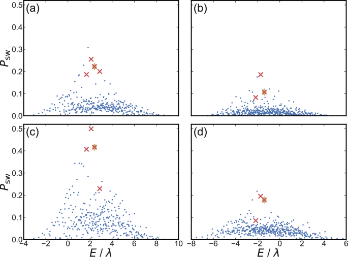
The weights of the ferromagnetic magnon bound state are shown in a and b while the weights of the anti-ferromagnetic magnon bound states are shown in c and d. The special states marked by QCNN have anomalously large weight on the subspace of a particular type of quasiparticle, compared to typical eigenstates. Other parameters are λ = J = 10Δ, a, c n_dw = 2, b, d n_dw = 3.

Full size image

Anti-ferromagnetic magnon bound state

We identify another component of special states, recognized by QCNN, which can be understood as quasiparticles of a short anti-ferromagnetic string, as depicted in Fig. 8b. In Fig. 9c, d, we plot the total weight of each eigenstate in the subspace of the shortest anti-ferromagnetic string. The results confirm that some marked states exhibit unusually large weights in these configurations compared to typical eigenstates. Restricting to the subspace of the four configurations shown in Fig. 8b, we can similarly write down an effective Hamiltonian:

The energy of the ground state and the first excited state are ({E}_{k}=-sqrt{{Delta }^{2}+2{lambda }^{2}(1pm cos (k/2))}). Since the energy of the first excited state is closer to the exact scar state, we present it with purple dashed curves in Figs. 6 and 7. The deviation of the antiferromagnetic magnon bound states from the exact eigenstates is greater than that of the ferromagnetic magnon bound states, leading to a smaller component contribution, as shown in Fig. 9.

It is worth emphasizing that there are also some integrable local modes found in this model in the low-energy regime⁴². They can be approximated by oscillators in a linear potential, which give rise to spatially localized modes. Such states with localized modes have a rather distinct nature compared to the tower of states in Eq. (2) that we use as training set. Indeed, these trivial states are not marked by the QCNN. The non-thermal states discussed in this section, in contrast, are situated in the middle of the energy spectrum.

Experimental demonstration on quantum device

We demonstrate the performance of our QCNN on IBM’s quantum hardware, with the training process carried out classically via noise-free simulations. We then prepare the exact scar state (| {{mathcal{S}}}_{1}left.rightrangle) using a shallow circuit, which is fed into the trained QCNN on the quantum device to evaluate its performance. To combat noise, we introduce a shallow general layer as a preprocessing step to enhance hardware efficiency. Furthermore, the learning circuit is optimized by reducing the number of two-qubit gates, improving overall implementation.

The circuit used to prepare the (| {{mathcal{S}}}_{1}left.rightrangle) state is depicted in Supplementary Note 2. The trained QCNN successfully identifies this state, achieving a success rate of over 99% in a noiseless classical simulation. The success rate observed on quantum hardware is presented in Fig. 10, which improves as the number of iterations in the learning process increases. However, due to the inherent noise in real-world quantum devices, the overall success rate is lower than that achieved in noiseless simulations.

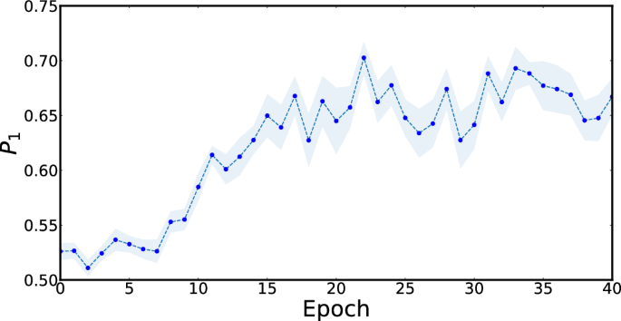
The experiment was conducted in 12 groups, each spaced hours apart to assess drift error. Each group involved 10⁴ measurement repeats to determine the success probability. Error bars indicated by the shaded region represent the standard error across different groups.

Full size image

To further enhance the performance of QCNN, we use error mitigation techniques to extrapolate to the noiseless limit. In particular, there is error from the state preparation circuit for (| {{mathcal{S}}}_{1}left.rightrangle), due to the imperfect two-qubit gates that implement non-local swaps. Our error mitigation technique uses two different methods to boost error, which yields a relation between error rate and the overall performance that can be used for extrapolation. The first method involves randomly adding single-qubit Pauli gates to multi-qubit gates, shown in Fig. 11a. The effect of such single-qubit errors can be simulated by Monte Carlo sampling. The second method uses the transformation (Uto U{left({U}^{dagger }Uright)}^{r}), as shown in Fig. 11b. In the noiseless situation, this is equivalent to applying a single unitary and hence has no effect on the result. On a noisy device, however, appending additional layers of U^†U increases the net error accumulated during the circuit evolution, and the performance becomes worse as the number of appended layers increase. Moreover, it can be directly implemented on the quantum device.

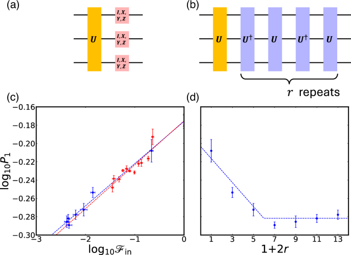
a, b Two different methods for boosting errors in the circuit: a adding single-qubit Pauli errors; b replacing U with (U{left({U}^{dagger }Uright)}^{r}). c Error mitigation according to input fidelity. Linear regression suggests P₁ ≈ 67 ± 1% in the limit of a perfect input state. The red and blue dots correspond to Monte Carlo sampling of single-qubit Pauli errors (averaged over 10³ noise realizations) and repeating U^†U, respectively. d Error mitigation according to error rate in the second approach. Linear regression using data prior to saturation suggests P₁ ≈ 63 ± 1% in the limit of a perfect input state.

Full size image

In Fig. 11c, d, we show results obtained using the two error mitigation methods discussed above. In Fig. 11c, we plot the success rate P₁ against the fidelity of the input state ({{mathcal{F}}}_{{rm{in}}}), for different error rates via either adjusting the rate of single-qubit errors, or adjusting the number of appended layers r in ({({U}^{dagger }U)}^{r}). The method for estimating ({{mathcal{F}}}_{{rm{in}}}) is detailed in Supplementary Note 2. Regression analysis in the log-log scale suggests that the success rate of the QCNN, in the limit of a perfect input state (| {{mathcal{S}}}_{1}left.rightrangle), reaches 67%. In Fig. 11d, we instead plot the success rate P₁ against the number of appended layers r in the second approach. By repeating the gates using (Uto U{left({U}^{dagger }Uright)}^{r}), the error is assumed to be 1 + 2r times that of U. The success probability decreases with increasing r and eventually saturates due to the finite size of the Hilbert space. Regression analysis before saturation suggests that the success rate of the QCNN, in the absence of input errors, reaches 63%.

Although experimental errors weaken the performance of QCNN, the classification signal is not completely drowned out by the noise. Our experimental results demonstrate that QCNN can still achieve a good success rate in the presence of noise, which we recover by using error mitigation. In this work we mitigate the state preparation noise, while the QCNN circuit error mitigation will be deferred to future works dedicated to full experimentation.

Generalizations to other models

In this section, we extend our QCNN-based approach to two additional models that host QMBSs. We begin with the PXP model, utilizing training data that include both analytically solvable and numerically identified scar states. Specifically, we incorporate the four exact scar states reported in ref. ³² and consider the states with the largest overlap with the (| {Z}_{2}left.rightrangle) across various energy windows as scar states³¹. Notably, the QCNN identifies many additional states as potentially non-thermal states, as shown in Fig. 12a. Some of these states exhibit smaller overlaps with (| {Z}_{2}left.rightrangle), remaining hidden within the chaotic spectrum. Inspired by ref. ⁴³, a symmetric subspace ({mathcal{K}}) can be constructed, which exhibits regular motion. The quasimodes within this subspace can be viewed as approximations of certain eigenstates. The subspace ({mathcal{K}}) is spanned by the basis states

where x represents the binary configuration of the spin chain, with the constraint that neighboring spins cannot both be in the “1″ state. Here, n₁ and n₂ denote the total number of “1”s at odd and even positions, respectively, and ({{mathcal{N}}}_{{n}_{1},{n}_{2}}) is the normalization factor. The Hamiltonian in this subspace is expressed as (langle {n}_{1},{n}_{2}| {H}_{{rm{xorX}}}| {n}_{1}^{{prime} },{n}_{2}^{{prime} }rangle). The eigenstates of quasimodes in this subspace are shown as yellow squares in Fig. 12a, and these quasimodes closely align with some of the marked states. In Fig. 12b, we plot the probability distribution of eigenstates within the subspace ({mathcal{K}}). Notably, the marked states have significant components within this subspace, demonstrating that the QCNN effectively learns hidden properties of the quasimodes without prior knowledge. Additionally, the QCNN not only identifies the top band in Fig. 12a, which is near the quasimodes, but also marks a second, lower band. This band has attracted considerable interest, though it still lacks a theoretical explanation.

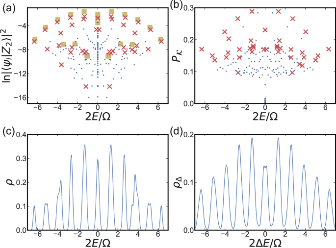
a Overlap between the eigenstates and the (| {Z}_{2}left.rightrangle) state, with red crosses marking the states identified by the QCNN. The yellow squares are the eigenstates of quasimodes in the symmetric subspace ({mathcal{K}}). b Weights of each eigenstates within the symmetric subspace ({mathcal{K}}). c Density of QCNN-identified states based in (a). d Density of energy differences between the QCNN-identified states in (a). In both (c) and (d), only states with non-zero overlap with the (| {Z}_{2}left.rightrangle) state are counted, with smoothing applied using Gaussian broadening of each points set to 0.1Ω/2.

Full size image

The dynamics of these states are governed by their energy spectrum. The marked states exhibit energies similar to those of the Z₂ tower states. These states form distinct energy towers, as depicted in Fig. 12c. Their energies are approximately equally spaced, as shown in Fig. 12d, indicating that their linear superposition can lead to stable oscillations.

The perturbations in the PXP model exhibit distinct behaviors. In cases where perturbations enhance quantum many-body scars^44,45,46, we observe a reduction in the number of non-thermal states identified by the QCNN. Under a uniform magnetic field perturbation, the QCNN additionally marks the second-highest energy band, alongside the top band, which is generally recognized as hosting scar states. Results for various perturbations are presented in Supplementary Note 3.

We also train the QCNN using the far-coupling Ising SSH model. The training data includes numerically solved scar states that exhibit significant overlaps with the Z₁₀₀₁ state³³. Due to the smaller number of scar states in this model compared to others with the same number of qubits, the accuracy of the QCNN is reduced. Nonetheless, the QCNN identifies several additional states, as shown in Fig. 13a. Some of these states have smaller overlaps with the Z₁₀₀₁ state. Although the peaks in the energy spectrum shown in Fig. 13b appear mixed and unclear, we can clarify their behavior by examining the energy spectrum in Fig. 13c. In Fig. 13c, the towers near ΔE = ±2.9J_e are primarily contributed by the scar states, whereas the towers near ΔE = ±1.2J_e are contributed by the additional states identified by QCNN. This suggests that the newly found non-thermal states exhibit a different oscillation frequency compared to the scar states.

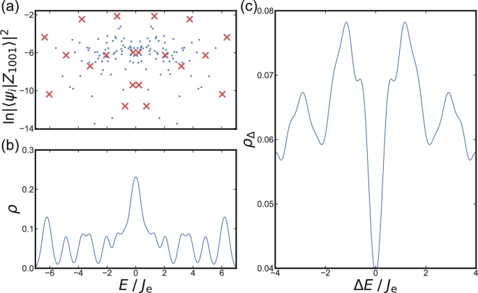
a Overlap between the eigenstates and the Z₁₀₀₁ state. The red crosses are states marked by QCNN. b Density of QCNN-identified states based in (a). c Density of energy differences between the QCNN-identified states in (a). In both (b) and (c), only states with non-zero overlap with the (| {Z}_{1001}left.rightrangle) state are counted, with smoothing applied using Gaussian broadening of each points set to 0.25J_e.

Full size image

We extend the QCNN approach to other models and discover additional states. The energy difference spectrum reveals that these identified states are non-thermal with relatively small dispersion. This demonstrates the QCNN’s capability to identify non-thermal states across various models. Analytical understanding of these non-thermal states, similar to that presented for the xorX model in this work, is an interesting open problem.

Recent advances in the use of QML to investigate scar states have garnered considerable interest, resulting in a variety of related research. Here, we discuss differences between their studies and our approach. For instance, ref. ²⁸ introduces a general classifier using quantum variational autoencoders, where each eigenstate is assigned its own learning circuit. This approach can be computationally expensive, with costs scaling exponentially as Hilbert spaces grow in size. In contrast, our method employs a single circuit to learn the common properties of known scar states, enabling the discovery of other similar states. This makes our scheme more computationally feasible. Meanwhile, ref. ⁴⁷ employs classical machine learning to detect single-body scar in billiard systems, given the classical description of eigenstates, but this methodology does not extend to many-body scars. ref. ²⁹ uses classical machine learning and dimensionality reduction techniques to minimize the distance among scar states, but this can lead to loss of quantum information. Although recent work shows that certain QCNNs can be simulated efficiently on classical systems⁴⁸, our QCNN differs in two key ways: (1) Our QCNN is enhanced with additional universal layers in front of the original QCNN. We anticipate that using a small number of these layers (scaling logarithmically or linearly with system size) will make classical simulation hard. (2) Preparing eigenstates of many-body systems remains a computationally challenging task. Scaling up system sizes will still rely on quantum hardware, complemented by techniques such as the variational eigensolver⁴⁹ for efficient eigenstate preparation.

The convolutional layers in QCNNs are designed to detect local patterns and correlations in quantum states, making them particularly effective for identifying scar states, which exhibit sub-volume law entanglement entropy. Scar states are well-represented by matrix product states (MPS)^32,50,51, which can be efficiently generated by tree-structured quantum circuits⁵². Given that QCNNs have an inverse tree structure, they are inherently well-suited for capturing the characteristics of scar states. Furthermore, the pooling operation in QCNNs parallels the coarse-graining step in the renormalization group (RG), simplifying the system while retaining essential information. Both QCNNs and RG employ multi-scale analysis to extract key features, albeit in different contexts²⁷. A deeper exploration of this correspondence and its underlying mechanisms remains an open avenue for further investigation.

In conclusion, the QCNN trained on scar states effectively identifies additional non-thermal states. Some of them primarily occupy a small fraction of the Hilbert space and can be approximately described as spin-wave modes of various quasiparticles. We construct effective Hamiltonians based on this framework, capturing key features of the exact many-body eigenstates. Additionally, we validate our approach on a quantum device, achieving a notable success rate with the use of error mitigation techniques. This study highlights the potential of QCNNs in uncovering hidden non-thermal states within the many-body spectrum, paving the way for future research into more complex quantum systems and their non-thermal behavior.

Enhancement of quantum convolutional neural network

Our approach utilizes QML by feeding known scar states as the training data set. However, scars are rare, as their number grows linearly with the number of qubits, whereas the Hilbert space expands exponentially. To address this limitation, we include superpositions of QMBS states in our training dataset, enhancing the model’s ability to learn from a small set of scar states.

For efficient training, we adopt QCNN as the quantum circuit ansatz. Its translational invariant gate architecture is well-suited for handling translational invariant Hamiltonians. Additionally, scar states can often be expressed as matrix-product states^32,51, which QCNN can learn efficiently.

As illustrated in Fig. 1, a QCNN is composed of convolution layers, pooling layers and a fully connected layer^24,53. Each convolutional layer consists of brick-wall two-qubit gates with identical parameters, reducing the number of parameters and facilitating more efficient classical optimization⁵⁴. These gates act as a quantum kernel, convolving the wave function through each layer. Furthermore, the locality alleviates the barren plateau problem⁵⁴. The pooling layers measure a subset of qubits after the quantum gates, reducing the number of operations needed in subsequent steps. This not only makes the quantum circuit shallower but also reduces noise. The fully connected layer then consolidates the information from the remaining qubits at the end of the process.

We further enhance the QCNN to improve its ability to classify quantum states with greater precision. Specifically, we introduce additional convolution layers after each existing convolution layer to enable the network to capture correlations over longer distances, analogous to the effect of using larger kernels in classical convolutional neural networks. The performance with different numbers of convolutional layers is shown in Fig. 14. To tackle more complex classification tasks, we introduce a few general layers of universal quantum gates to preprocess the input data. This adjustment helps handle finite-size effect and outliers which breaks translational-symmetry, such as disorders or boundaries. Furthermore, we incorporate an ancillary qubit initialized in the (| 0left.rightrangle) state, analogous to the zero padding at the boundary pixels in classical convolutional neural networks. This allows us to perform classification operations without altering the size of the Hilbert space (see Supplementary Note 1)

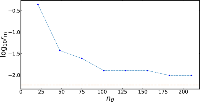
The rate of marked states r_m is the ratio of marked states to the total dimension of the Hilbert space. Each point represents a distinct set of circuit parameters and a corresponding training iteration. The orange dashed line indicates the rate of marked (scar) states in the input data. The system consists of 12 spins. The number of trainable parameters is given by n_θ = 12 + 3(9n_l + 3), where n_l is the number of convolutional layers preceding the pooling layers.

Full size image

When the circuit has too few layers, its limited discriminative power causes various states to become indistinguishable. As the number of parameterized gates increases, the classification error gradually decreases. This improvement may lead to overfitting in an over-parameterized circuit. The rate of marked states (i.e., those identified as scar states by the QCNN) tends to align with the rate in the input data, as shown in Fig. 14. Classification becomes saturated when the number of parameters approaches the size of the Hilbert space. The states identified by the circuit will transition between exact scar and chaotic states, with this transition expected to be continuous, akin to the classical case. In other words, the number of parameters controls the proximity of the regime to the exact scar states that are marked^19,29. Our study focuses on this transition to identify previously unknown non-thermal states with scar-like characteristics.

Training with scar states

To train the enhanced QCNN, we use training data generated from known QMBS states. Specifically, for a system with known scar states, we label these known scar states and their superpositions as y_i = 1, while labeling other eigenstates and their superpositions as y_i = 0. We then randomly select an equal number of states from each label category and train the enhanced QCNN using gradient descent to minimize the loss function⁵³

where d is the total number of input states, and q_i denotes the probability of the output qubit being in (| 1left.rightrangle) state. This q_i also corresponds to the single-shot measurement accuracy for identifying exact scar states. The enhanced QCNN is expected to distinguish scar states from thermal states after sufficient training with enough number of layers. After training, we evaluate the QCNN’s performance by testing it on the eigenstates of the Hamiltonian. For convenience, we consider an eigenstate to be “marked” if the output q_i exceeds 50%, matching the rate of scar states in the training set. Experimentally, this classification is achieved through a majority vote across multiple trials and measurements³⁷. In this context, achieving zero loss indicates perfect classification, although zero classification error does not necessarily imply the loss function fully decays to zero. The loss function also reflects the model’s robustness to noise.