Understanding spring forecast El Niño false alarms in the North American Multi-Model Ensemble

Introduction
Given El Niño’s global impact on weather and climate, including extreme weather and global agricultural production, there is significant value to accurate forecasts at longer leads1,2,3,4,5. El Niño forecasts have always been tricky during the boreal spring (from March to May), a period known as the spring predictability barrier6. The spring predictability barrier has been theorized to result from air–sea interaction, upper-ocean advection, thermocline-mixed layer processes, or cloud feedback processes amongst other physical mechanisms7,8,9. Statistically, it coincides with a sharp drop in autocorrelation of SST anomalies. Due to El Niño’s global impact, there have been attempts to improve El Niño predictions from boreal spring and earlier since the advent of seasonal predictions6. In a statistical context, warm water volume shows the most skill during this time10,11. But, even though warm water volume holds some predictive value during the spring predictability barrier, large springtime warm water volume anomalies do not guarantee an El Niño event in the following winter12,13. Recent research has also pointed to subsurface velocity and salinity as representing some additional skill at or through the spring predictability barrier14,15. These metrics align with the theoretical understanding of the oscillatory nature of El Niño-Southern Oscillation (ENSO) and pre-conditions for an El Niño event.
Factors beyond the tropical Pacific have also been explored for their impact on El Niño forecast skill. Regions external to the tropical Pacific that have been shown to impact El Niño forecasts include the North and South Pacific Meridional Modes, Indian Ocean SSTs, the Indian Ocean Dipole, and the tropical Atlantic16,17,18,19,20,21,22,23,24,25. Some other regions also have been noted for their ability to predict though the spring predictability barrier26. Tropical regions can influence the tropical Pacific through changes in background Walker circulation or enhanced Madden-Julian Oscillation (MJO) propagation. Connections from extra-tropical to tropical regions typically occur through the wind-evaporation-SST feedbacks transporting anomalies equatorward and leading to additional westerly wind forcing in the western and central equatorial Pacific27,28. Other forecast techniques, such as using model analogs, have also demonstrated similar or higher skill in predicting El Niño through the spring predictability barrier29,30,31. This suggests that there is room for improvement in the dynamical forecast models’ prediction of El Niño.
Here, we focus on the utilization of dynamical seasonal forecast models and their El Niño forecasts. Although dynamical seasonal forecast models offer valuable guidance for ENSO forecasts, they, like other methods, encounter challenges with the spring predictability barrier6. Additionally, in the last decade, there have been a number of high-profile El Niño forecasts where the forecast models have been very confident in the formation of an El Niño event but an El Niño event did not occur32,33,34. Previous studies have explored single models and specific circumstances and found that there were occurrences of “excessive momentum” that produced these over-confident forecasts35, however, there has not been a systematic multi-model study of these failed confident forecasts, nor, has there been confirmation that these forecasts are truly an issue and not just a representation of recency bias. Here, we explore the North American Multi-Model Ensemble (NMME) phase II36 set of 6 models and 30 years hindcasts for El Niño forecasts that failed despite high confidence and our goals is to quantify the frequency and to understand the causes of the forecast bias.
Results
Occurrence of confident successes and false alarms
As a first step, we examine all the February, March, April, and May initialized hindcasts from NMME to see if the models are predicting El Niño and La Niña events with the appropriate levels of confidence. To do this, for each model, we bin each forecast into quartiles based on the percentage of ensemble members predicting an El Niño or La Niña averaged over leads of 180–270 days and compare it with the frequency of observed El Niño or La Niña events from all of the forecasts in each bin (Fig. 1a and b, respectively). These figures show that for the most confident El Niño forecasts (>75% confidence), do not result in El Niño events at the expect rate for that level of confidence. Using slightly fewer or slightly more bins does not change this result. For confident La Niña forecasts, the forecast confidence does match the observed frequency. Even though they are not the optimal tool for evaluating forecast overconfidence, we also examine the Receiver Operating Characteristic (ROC) for El Niño forecasts (Fig. 1c). Unlike reliability, ROC is evaluated on 10% forecast confidence intervals since the entire set of 120 forecasts are evaluated for hit rate and false alarm rate at each threshold. One important advantage of ROC is that there is not a concern of splitting the sample up into to too many different bins. Since the minimum number of ensemble members is 10, using 10% intervals for ROC shows the most information with the least repetition. On the left hand side of the ROC diagram, where the highest confidence forecasts are evaluated, for at least half of the models the hit rate decreases much more rapidly than the false alarm rate. This is consistent with forecast overconfidence for high-confidence forecasts observed in the reliability diagrams. Thus, there is a model over-confidence problem for forecasting El Niño events but not for forecasting La Niña events and for the rest of this paper we will focus on just El Niño forecasts.

Model reliability diagram for boreal spring for a El Niño and b La Niña forecasts with a 6–9 month lead. c Receiver operating characteristic for spring El Niño forecasts for each model. The Hit Rate and False Alarm are calculated using a 10% forecast confidence is the threshold for an event forecast in the upper right hand portion of the figure and increase that threshold by 10% for each point as the curves travel down and to the left, ending with a 100% forecast confidence in the lower right.
Based on these results, we identify the confident El Niño forecasts (more than 75% of a models’ ensemble members predict an El Niño event) and divide them into false alarms (no El Niño event) and confident successes (El Niño event). To better account for factors that could lead to a missed forecast, including early or late onset and delayed transition, a broader range of forecasts are examined and categorized into confident success and false alarms for the rest of this paper (see “Data and methods” for more details). Figure 2 shows the distribution of the confident successes and false alarm forecasts across the different models in the hindcast from this updated process. The outcomes from the updated process are summarized by model in Table 1. Out of the 120 hindcasts in this study, the different models range from a low of 19% of the forecasts are confident forecasts (GEOS5 and CCSM4) to a high of 33% (CanCM4). The confident forecasts are successful between 53% (CanCM3) and 79% (CFSv2) of the time. Given the minimum threshold of 75% of the ensemble members predicting an El Niño event for a confident forecasts, we would expect the models to be correct at least 75% of the time for these selected forecasts. However, only one model (CFSv2) exceeds this threshold, implying that the individual forecast models do have an El Niño false alarm problem. This is highlighted by the reliability diagram in Fig. 1a).

All of the spring forecasts in for each model from the hindcast period placed into the confident success, false alarms categories. Confident forecasts are where >75% of the ensemble members predict an El Niño event. Confident successes are where these confident forecasts are successful and false alarms are where the confident forecasts do not verify.
We can also explore how frequently each model makes confident El Niño forecasts. During the hindcast period, there are nine observed El Niño events, making climatological rate of occurrence 30%. However, due to the spring predictability barrier, we would expect that there should not be frequent confident forecasts for the forecasts initialized then. Studies examining forecasts of individual El Niño events and misses also give a wide range of outcomes for those specific events. Therefore, our prior is that springtime confident forecasts should happen at a much lower rate than the 30% occurrence rate. However, two out of the six models produce confident El Niño forecasts in excess of 30% of the time and three of the six models produce confident forecasts in excess of 25% of the time from spring time initializations. To test the likelihood of such confident predictions, we use the conceptual recharge oscillator model of Levine and McPhaden8,12 to determine the likelihood of this many confident forecasts in a 30-year hindcast. We run 1000 30-year hindcast experiments that mimic a single model in NMME in this conceptual model (details of the model and method can be found in the “Data and methods” section). In the conceptual model, we test three different combinations of noise forcing and growth rate to sample across different levels of deterministic forecasts. Since we are simulating ENSO as a damped driven oscillator, a decrease in λm corresponds to an increase in growth rate and a less damped ENSO. To offset the increase in growth rate on ENSO amplitude, the state-dependence of the noise, B is decreased. This combination of changes to growth rate and noise creates a more deterministic ENSO. Conversely, to simulate a less deterministic (More Damped) ENSO, λm and B are increased. Yet, even in the most deterministic case (Less Damped), the frequency of confident forecasts for the least confident of the NMME models lies in the tail of the distribution making it exceedingly unlikely that the NMME models are correctly estimating El Niño forecast spread (Fig. 3). Therefore, it is likely that model overconfidence in its springtime predictions contributes to the number of false alarm forecasts. Generally, the models with the largest number of confident forecasts have the largest number of false alarms.

Histogram of confident forecasts for 1000 hindcast experiments and density estimate for each conceptual model configuration. Values of the individual models are shown as black vertical lines. The multi-model ensemble is the thick vertical line. These decimals here are the same as the Confident percentage column of Table 1.
Moreover, these problems remain unresolved even when employing a multi-model ensemble. While the multi-model ensemble has fewer confident forecasts than any individual model, the number of confident forecasts is not much lower than the lowest of the contributing models. In addition, the multi-model ensemble false alarm fraction is higher than about half the models and still well below 75%. A closer examination of Fig. 2, also shows that many of the models produce false alarm forecasts at the same time, suggesting that there are potential commonalities for false alarms across the models that we will explore further through this manuscript.
Common elements of a confident forecast
Given our understanding of equatorial heat content as a necessary, but not sufficient condition for El Niño events13, we explore its role in producing a confident forecast. Due to the two-layered nature of the tropical ocean, sea surface heights (SSHs) and the depth of the 20° isotherm are often used as proxies for the upper ocean heat content. However, analyzing these quantities can sometimes lead to slightly different descriptions of the variability of the heat content in the upper ocean. Here, consistent with previous studies37,38 and based on the fact that SSH derived from altimeter data primarily reflect the motion the main thermocline39,40, we have used SSH data produced by the Global Ocean Data Assimilation System (GODAS) as a proxy for the variability of upper ocean heat content. SSH tend to be above normal during initial months for those confident forecasts (Fig. 4). Further, the pattern shows a broad deepening anomaly in the western Pacific and a more equatorially bound positive anomaly across the rest of the Pacific Ocean. When comparing confident forecasts to the rest of the forecasts, the positive anomalies in the western Pacific play a more prominent role in distinguishing the confident forecasts from the rest compared to the whole basin SSH. These results align with the findings of Planton et al. and Izumo et al.41,42 regarding the significance of western Pacific warm water volume as predictors through the spring predictability barrier. However, SSH anomalies show limited ability to separate the confident successes from the false alarms. This aligns with the idea that while high heat content is important for El Niño, it is not sufficient on its own to produce an El Niño event12. As shown in Fig. 4, many forecasts initialized with high heat content do not confidently predict an El Niño event. Therefore, we examine other proposed El Niño predictors in the dynamical forecast models to see if they contribute to confident El Niño forecasts.

a Composite of GODAS SSH anomalies for the initialization of all confident forecasts. Box outlines 140W-180, 5S-5N. b Distribution of all sea surface height anomalies by forecast type.
Previous studies of false alarm El Niño forecasts have also highlighted what they have termed as the “momentum problem”. This refers to the tendency of the models to predict further anomaly growth and an El Niño event when the Niño region SST anomalies are increasing. This issue is particularly present during the boreal spring35. Thus, we next examine the role of this sea surface temperature anomaly change, adopting the momentum terminology from Tippett et al.35 in the context of this study. To do this, we analyze the change in SST anomalies from one month prior to model initialization to the month of model initialization (SST anomaly tendency) (Fig. 5). In confident El Niño forecasts, significant warming is observed across the entire cold tongue region during the month prior to forecast initialization. In Fig. 5b, the Niño3.4 region SST tendency distribution is shown. This confirms previous studies that show that positive SST tendencies at the beginning of the forecast are common in failed high-confidence El Niño forecasts35. However, similar to the SSH anomalies, when considered individually, positive SST anomaly tendency, on its own, is not prescriptive of a high confidence forecast.

a Composite of 1-month SST tendency for the month prior to forecast initialization for all confident forecasts. Boxes show 3 Niño regions and NE Pacific region. b Distribution of all SST tendencies by forecast type.
When combined together, a forecast, initialized with positive SSH anomalies and a positive SST tendency, is very likely to be confidently headed towards an El Niño event (Fig. 6). As shown in Fig. 6, the joint pdfs of the forecasts with positive SSH anomalies and positive SST anomaly tendencies for confident forecasts occupies a small region in the upper right quadrant of the total joint pdf, leading to very few forecasts with both positive tendencies and high heat content anomalies that do not produce confident forecasts. However, these two initial conditions of the forecast are not determinate of whether the forecast will be a false alarm or not as there is substantial overlap between the confident successes (green) and false alarms (orange) in Fig. 6. To separate out the false alarm forecasts from the other high confident forecasts, additional information is necessary.
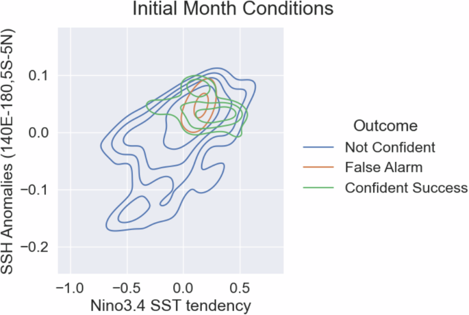
Joint distribution of sea surface height and temperature tendency by forecast type. Contours represent the frequency of events outside the contour, which increases by 20% per level. The lowest contour is at 20%.
Separating successes from false alarms
Neither the positive SSH anomalies nor the equatorial SST tendencies are capable of separating the successful confident forecasts from the false alarms. To look for differences between the confident successes and the false alarms, we composite the model forecasts for the first 15 days of surface air temperature anomalies between the confident successes and the false alarms. Figure 7 shows that, in cases of confident successes, the surface air temperature anomalies in the northeast and southeast subtropical Pacific are higher than in the cases of the false alarms. The anomalies are located in regions of the Pacific Ocean that coincide with the maximum centers of the North Pacific Meridional Mode and the South Pacific Meridional Mode. Positive SST anomalies in both meridional modes have previously been shown to influence El Niño development16,19,43,44,45.

Multi-model composite of initial 15 days surface temperature anomaly for a confident successes and b false alarms. Boxes highlight Niño regions, North-East and South-East Pacific regions.
We further analyzed the PDFs of confident successes and false alarm forecasts in these two regions and found a clear difference. Confident successes and false alarms are characterized by surface air temperature anomalies higher than normal in the north Pacific, while in cases of false alarms, surface air temperature anomalies are lower than normal in the north Pacific (Fig. 8). Such clear separation does not occur based on anomalies in the southeast Pacific. The difference in results between the north Pacific and south Pacific may be due to the time of year when either mode has its peak impact El Niño development. The north Pacific meridional mode impacts El Niño during the period we are considering and the south Pacific meridional mode impacts El Niño later in the El Niño growth phase, during the austral winter months (JJA)19,46. We note that the anomalies in the north Pacific are important for distinguishing confident successes from false alarms, the anomalies in both cases are not particularly outside the distribution of temperatures in non-confident forecasts. This suggests that while the extra-tropical temperatures, and likely the north Pacific Meridional Mode, is important for forecasting El Niño events, there are other factors that play a significant role in accurately forecasting El Niño events.

Initial temperature anomaly distributions for a north-east tropical pacific and b south-east tropical pacific surface temperature.
The findings indicate that the confident forecasts often stem from equatorial Pacific forcings, while false alarm forecasts differ from the confident successes due to extra-tropical forcings. It suggests that the forecast models are struggling to correctly simulate tropical processes involved in El Niño development to the exclusion of important extra-tropical processes. While shown specifically here for the North Pacific Meridional Mode, this study does not rule out that other forms of predicable extra-tropical variability47,48 are being ignored by the dynamical models. When the forecast models correctly succeed, the result is correct not because the model is better, but rather this is an El Niño event that should be confidently forecast.
Tropical mechanisms
The meridional modes influence El Niño by transporting changes in the trade winds from the extra-tropics to the tropics, eventually weakening the tropical trade winds and supporting an El Niño event18,28. While the north Pacific Meridional Mode is crucial for distinguishing confident successes from false alarms, the lack of influence of the meridional modes on the confident forecasts may still have roots in the model representation of the tropics. Returning to the tropics, we revisit the entire set of boreal spring forecasts. The fact that temperature tendency is an important factor in producing the confident forecasts along with recognizing that El Niño is a weakly damped mode of tropical Pacific variability gives rise to the question: Is the model forecast El Niño damped enough or does the positive Bjerknes feedback too easily escalate slight warmings into full El Niño events? This is particularly important for the boreal spring where seasonal analysis of El Niño stability shows that ENSO stability is trending from stable to unstable ahead of summer, making predictions particularly challenging8,49. Without doing a full stability analysis here, we analyze the one-month change in temperature anomalies in the different Niño regions in the models and reanalysis as a function of starting temperature anomaly for the first month of the forecast (average of days 30–45 minus average of days 0–15). In all the Niño regions, the regression coefficient for the 1-month tendency as a function of initial anomaly is negative confirming that the anomalies are damped as expected (Fig. 9). However, two-thirds of the models have less negative slopes and are therefore less damped than the observations (black line). This disparity is more pronounced in the Niño3.4 region than in the Niño4 region, suggesting that the models’ Bjerknes feedback might be too strong.

One month temperature change as a function of temperature anomaly for a Niño 4 region and b Niño3.4 region. The black line in both plots is from ERA5.
The Bjerknes feedback in the tropical Pacific is the weakening of the trade winds in response to warming SSTs in the equatorial cold tongue, which in turn further warms the SSTs and then further weakens the trade winds. This weakening of the trade winds and westward shift of warm waters in accompanied by a westward shift of precipitation. Changes in rainfall pattern are a key signal of ENSO evolution. We focus on precipitation anomalies along the warm pool edge (between 150E-180) and how they relate to the initial Niño4 temperature anomalies (Fig. 10). Using a 15-day window, the precipitation anomalies in many of the models are still significantly correlated with initial Niño4 temperature anomalies. In most models, the contemporaneous correlations are too strong compared with observations. These correlations remain too large for the first few months in many models. The models that show the largest change and a shift to a significant negative correlation (CanCM3 and FLOR-B01) both have the highest percentage of confident forecasts that fail and the model that most underestimates the correlation (CCSM4) has the fewest confident forecasts. However, if the SST anomalies were correctly damped, then the future precipitation anomalies would also not be connected to the initial Niño4 anomalies. To quantify the difference in the dependence of the modeled relationship between precipitation on initial SSTs, we calculate the root-mean-squared error (rms) of the model correlation over time from the observed correlation. Figures 10c and d, show the rms error for each model compared with the confident forecast rate and the percentage of successful confident forecasts, respectively. The models that do the best at capturing the decay of the dependence of the precipitation on the initial temperature anomaly have both fewer confident forecasts and are their confident forecasts are correct more frequently.

a Regression of precipitation on Niño4 temperature anomalies for CMAP/ERSST. Box shows the warm pool edge region (150E-180, 5S-5N). b Correlation for 15-day segments of precipitation anomalies with initial Niño4 temperature anomalies. The black line is the correlation between ERA5 and CMAP. c Root-mean square error of precipitation correlation from models with observed temperature and precipitation lag correlation and confident forecast rate. d Root-mean square error of precipitation correlation from models with observed temperature and precipitation lag correlation and false alarm fraction.
Discussion
We analyzed the boreal spring NMME El Niño forecasts for confident forecasts of the upcoming El Niño. These forecasts predicted El Niño events at a higher rate of confidence than they actually occurred at during the 30-year hindcast period. Consistent with previous studies, the confident forecasts occurred in the models initialized with a positive equatorial warm water volume and positive tropical SST tendencies. The warm water volume anomalies are consistent with expectations from previous studies on ENSO theory10,32 and studies of El Niño prediction during the boreal spring8,13. The SST tendency is consistent with previous studies on El Niño false alarm forecasts35. The confident forecasts fail to verify when the extra-tropical north Pacific does not support the generation of an El Niño event, most likely through processes associated with the north Pacific Meridional Mode18. An analysis of why the warm water volume and temperature tendency tend to overestimate the El Niño confidence shows that the equatorial Pacific SST anomalies are not damped strongly enough in the models compared with observations. This is the likely result of an overly deterministic precipitation response to warming of SSTs along the Western Pacific Warm Pool edge and subsequent too strong Bjerknes feedback. Therefore, we find that the dynamical forecast model confident forecasts succeed in spite of the models themselves, not because they are correctly simulating influences on ENSO outside of the tropical Pacific, but rather because they are producing too many confident forecasts and the model is only coincidentally correct when the forecast should be confident.
In general, the seasonal forecast models seem to be overly reliant on the tropical Pacific and underestimate the impact of other processes for boreal spring El Niño predictions. Yet, the forecast models tend to have generally accurate ENSO predictions outside of the types of forecasts analyzed here6. To understand how this might come about, we can look at a conceptual ENSO model for some clues. Using a simple recharge oscillator model, if the ENSO growth rate is too strong, then the corresponding external forcing or noise forcing terms would need to compensate by being too weak in order to get El Niño amplitude correct. However, because of how the forecast spread evolves differently with the growth rate and noise forcing, the forecast spread would be too small and the uncertainty in the forecast underestimated50. This leads to overconfident forecasts and this framework for understanding El Niño and its forecasts is consistent with the results presented here. Comparison with studies that use a similar theoretical framework provides an explanation for why this a problem with El Niño forecasts and not La Niña forecasts8,51. The inclusion of state-dependent noise forcing in a recharge oscillator model decreases El Niño predictability without impacting La Niña predictability and could explain the difference in predictability between forecast models and theoretical studies23,30. Furthermore, the recharge oscillator with state-dependent noise framework may also provide additional guidance for improving confident El Niño forecasts in dynamical forecast models52 found that the state-dependent component of the noise forcing of ENSO was under-represented in CMIP3 and 5 models, which was connected to the cold tongue bias. Recent work in CESM1, a model that is used both for climate projections as well as seasonal forecasts, found that reducing the cold tongue bias improved ENSO forecasts53. While the cold tongue bias is a long extant problem in coupled climate modeling, we are optimistic that improvements in its representation will also improve El Niño forecasts. Future work will explore which processes and feedbacks for ENSO are important for the over-confidence in El Niño forecasts and the role of different influences of uncertainty in El Niño forecasts should and do play a role in the seasonal forecasts.
Data and methods
The six models used in this study are CanCM3, CanCM4, CCSM4, CFSv2, FLOR-B01, and GEOS5. These six models all participated in the North American Multi-Model Experiment (NMME) Phase 236. Details about the model configurations can be found in Kirtman et al.36. The 30-year hindcast period is from 1982 to 2011. Anomalies are defined from each models’ individual climatology based on start month and lead from the entire hindcast period. Both CFSv2 and CCSM4 have split climatologies before and after 1999 based on changes to the source of initial conditions54. The models were chosen due to their data availability for daily resolution seasonal forecasts for surface air temperature and precipitation. There is less availability in the archive for sea surface temperature and surface winds or wind stress. ERA5 daily reanalysis surface 2m air temperature is used for comparison with model surface temperature and CMAP pentad precipitation is used for comparison with precipitation55. ERA5 surface temperature is compared to more traditional SST products for El Niño observations, ERSSTv5 and OISST and using 15-day averages there are few differences56,57. For sea surface height data, GODAS ocean reanalysis is used58.
Model forecasts initialized in months February, March, April, and May are used in this study. With the exception of CFSv2, the forecast ensembles are all from the first of the month. CFSv2 produces one forecast on the synoptic hours (0z, 6z, 12, z 18z) every five days to create it’s ensemble. CFSv2 forecasts are grouped into the month they are initialized in for purposes of defining its ensemble. For Fig. 1, the models’ forecasts are initially evaluated using 180–270 day (6–9 months) lead forecast averages, so February initialized forecasts target August to October. Following this initial analysis, perspective confident El Niño forecasts are defined as a forecast where at leads greater than 90 days, the 45-day average Niño3.4 temperature anomaly exceeds 0.5 degrees in 75% of the ensemble members. For the multi-model ensemble, a confident forecast is when the average confident forecast fraction across the six models exceeds 75%. Confident forecasts are then split into successes and false alarms based on whether an El Niño event occurred during the forecast period. Each perspective confident success and false alarm was then visually examined to confirm the forecasts were for El Niño events and that the observations did or did not reach El Niño status during a different portion of the forecast period.
Conceptual model
The recharge oscillator model is a widely used conceptual model of ENSO. Here, we use a similar version to that used in Levine and McPhaden8,12, both studies on ENSO predictability. The model equations are:
where T is surface temperature anomaly in the Niño regions, h is heat content anomaly, and ξ is noise forcing. For the noise forcing, r = 8 and w(t) is gaussianly distributed white noise, producing Gaussian red noise with a decorrelation timescale of 45 days. The noise forcing has a standard deviation σ = 4.3 years−1 and is modified by a state-dependent term ((B{mathcal{H}}(T))) where ({mathcal{H}}) is heaviside function defined by ({mathcal{H}}=0) if T < 0 and ({mathcal{H}}=1) if T ≥ 0. The growth rate, λ, is split into two components, it’s mean, λm, and the amplitude of it annual cycle, λAC. In the middle of the road experiment, λm = 2 and B = 0.3. In all experiments, λAC = 2.5 and ωa produces a 360-day year. Twelve 30-day months are assumed. The natural frequency for ENSO, ω = 0.25 years−1. For justification of these parameters, see Levine and McPhaden12 and references cited therein.
To produce each hindcast confident forecast distribution, we run a 10,000-year-long integration of the model. From this long integration, we randomly select 1000 30-year periods. For each 30-year period, we select the initial conditions corresponding to February 1, March 1, April 1, and May 1. For each of these 120 initial conditions, we run a 1-year forecast with 10 ensemble members. If greater than 75% of the ensemble members for a given forecast produce an El Niño event (45-day average exceeds one standard deviation of the long integration temperature at a time beyond 135 days), then the forecast is considered confident that an El Niño will form. The whole experiment is run twice more under less damped and more damped conditions. In these experiments, λm = 1.5 and B = 0.05 and λm = 2.5 and B = 0.55 for the more and less damped experiments, respectively. These values of λm and B are chosen to keep the standard deviation of the long integrations approximately constant. The values of B are approximately the best guess and uncertainty ranges calculated from observations by Levine and Jin59.


Responses