Understanding the microscopic origin of the magnetic interactions in CoNb2O6

For more than a decade, the quasi-one-dimensional Ising ferromagnet CoNb₂O₆ (Fig. 1) has been considered as a good experimental realization of the transverse-field ferromagnetic Ising chain (TFFIC)^{1,2,3,4,5,6,7,8,9,10,11,12}, showing the expected features of a transversal-field-induced quantum critical point at 5 Tesla between a magnetically ordered and a quantum paramagnetic phase. At the critical field, the spin excitations change in character from domain-wall pairs in the ordered phase to spin-flips in the paramagnetic phase^6,10. Such a scenario has been confirmed by inelastic neutron scattering (INS)^6,13,14, specific heat¹⁵, nuclear magnetic resonance (NMR)¹⁶ and THz spectroscopy^17,18,19,20 experiments. These early studies of CoNb₂O₆ were largely interpreted in terms of bond-independent XXZ-type anisotropic couplings, following expectations from classic works on Co²⁺ magnetism^21,22.

Co²⁺ zigzag chains expanding along the c-axis. The octahedral oxygen environment of the Co-ions is visible. The Co²⁺ chains align antiferromagnetically to each other forming an antiferromagnetic system.

Full size image

However, while the dominant physics of CoNb₂O₆ can be described by the TFFIC model, a (symmetry-allowed) staggered off-diagonal exchange contribution was proposed to be required to capture the details of the INS spectrum¹⁰, and a further refined TFFIC model was recently extracted from fitting to the INS spectrum at zero and high fields^13,14. A similar assertion was made on the basis of the field-evolution of the excitations in THz spectroscopy¹⁹, with the authors favouring an alternative twisted Kitaev chain model²³ to parametrize the bond-dependent interactions. The latter model was motivated, in part, by proposals of possible Kitaev-type bond-dependent couplings in high-spin Co²⁺ compounds^24,25,25,26, provided that a specific balance between competing exchange interactions is met. These proposals are in analogy with important developments in the last decades on the nature of exchange interactions in spin-orbit-coupled 4d and 5d transition-metal-based magnets in the context of bond-dependent Kitaev models^{27,28,29,30,31,32,33,34}. At present, the validity of this scenario for specific Co²⁺ materials and the role of different exchange contributions remains a subject of discussion across multiple Co²⁺ materials^{35,36,37,38,39,40,41,42,43}. Adding to the discussion of CoNb₂O₆, recently ref. ⁴⁴ evaluated the various exchange terms in the spin Hamiltonian through a perturbation theory study and refitting of the experimental spectra. Furthermore, based on symmetry arguments, the authors of ref. ⁴⁵ provided valuable insights into the general structure of the spin-anisotropic model of CoNb₂O₆ and studied effects of magnon interactions in its excitation spectrum by adopting the model parameters from ref. ^13,14.

In reality, the various experimentally motivated parametrizations of the couplings in CoNb₂O₆ lead to similar Hamiltonians, but the apparently conflicting interpretations call for a detailed microscopic analysis of the exchange contributions.

In this work, we present a detailed study of the exchange interactions in CoNb₂O₆, obtained by applying an ab-initio approach with additional modelling that accounts for various drawbacks of a purely density functional theory (DFT)-type ansatz.

The method allows us to extract and understand the origin of the magnetic couplings under the inclusion of all symmetry-allowed terms, and to resolve the conflicting model descriptions above. We find that both experimentally proposed models are only then consistent with a microscopic model if this model incorporates a dominant ligand-centered exchange process, which is rendered anisotropic by the low-symmetry crystal fields environments in CoNb₂O₆, giving rise to the dominant Ising exchange. The smaller bond-dependent anisotropies are found to arise from a combination of terms we discuss in detail. We demonstrate the validity of our approach by comparing the predictions of the obtained low-energy model to measured THz and INS spectra. Finally, this model is compared to previously proposed models in the perspectives of both TFFIC and twisted Kitaev chain descriptions.

Magnetic Exchange Couplings

All results for the magnetic exchange couplings presented in this section are obtained using projED, an ab-initio based method. The detailed description of this approach can be found in the “Methods” section.

CoNb₂O₆ has been discussed both, in terms of a twisted Kitaev chain as well as an Ising model supplemented by isotropic and anisotropic couplings (see “Methods” section)^{6,13,14,19,44,45}. The former perspective is made apparent in the cubic xyz coordinate system of Fig. 2a, while the latter is natural in the principal XYZ-coordinates of Fig. 2b.

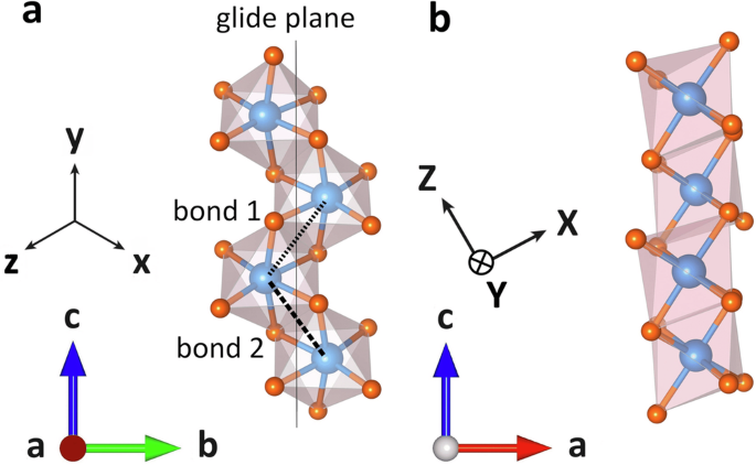
Different coordinate systems shown in a Co-chain with surrounding oxygen octahedra. Due to the antiferromagnetic alignment of the chains the local coordinate systems depend on the choice of the chain. a Cubic axes x, y, z. They correspond to the conventional Kitaev coordinates. The glide plane perpendicular to the crystallographic b-axis is visible, as well as the two bonds defined in the twisted Kitaev notation. Bond 1 is perpendicular to the x-axis, bond 2 to the z-axis. b Principal axes X, Y, Z as described in Eq. (8) for ϕ = 30°.

Full size image

Following Fig. 2a, bond 1 is defined as perpendicular to the cubic x-direction and bond 2 perpendicular to z. Because of an inversion center in the center of each bond, the Dzyaloshinskii-Moriya interaction vanishes, and the symmetry-allowed magnetic exchange on bond 1 can be cast into the form

in cubic xyz-coordinates. Here, K is the Kitaev coupling, J_K is conventional Heisenberg exchange, and Γ_i are off-diagonal symmetric couplings. The exchanges on both bonds are related through a glide-plane symmetry:

which implies for the second bond:

An alternative parametrization of the Hamiltonian is given in terms of the principal XYZ-axes of Fig. 2b and Eq. (8) with ϕ = 30°:

with odd numbers of i on bond 1 and even ones for bond 2. Within this parametrization J represents the overall scale of the couplings.

The details of the transformation between one parametrization and the other are presented in Supplementary Note 3.

As discussed in detail in refs. ^24,25,26, there are two main categories of contributions to the magnetic exchange. The first involves all of those processes that can be downfolded into kinetic exchange processes between d-orbital Wannier functions, arising at order t² in the downfolded d-only picture. These terms include the main contribution to the bond-dependent anisotropic exchange terms. The second category of contributions are ligand-exchange terms, involving the mixture of the ground state j_1/2 configurations with excited states having two holes in different p-orbitals on the same ligand. When downfolded into the d-orbital basis, such contributions appear as effective intersite Hund’s couplings in the electronic Hamiltonian. In the low-energy spin model, they produce ferromagnetic intersite couplings with an anisotropy that is essentially bond-independent. This anisotropy originates from the specific spin-orbital composition of the single-ion states, as revealed in the anisotropy of the g-tensor.

In our numerical approach, discussed in the “Methods” section, we make an explicit approximation for the downfolded intersite Coulomb terms, the strength of which is controlled by a scaling parameter γ, such that ({{mathcal{H}}}_{{rm{nn-U}}}propto gamma). This represents the renormalization of the ligand p-orbital Coulomb interactions relative to free ion values. Over a range of different 3d compounds, we have found empirically that γ values in the range 0.6–0.8 typically reproduce well experimental responses (see, for example,⁴⁶). We therefore perform the projED calculation of the low-energy couplings for a range of γ values. Figure 3 displays the development of the magnetic couplings with varying γ for the range γ = 0.55 to 0.65. Here we considered the parametrization given in Eq. (4). The nearest neighbor couplings are always ferromagnetic, with a dominant Ising anisotropy for the entire range of reasonable γ values. μ_XY and μ_ZY have matching signs that alternate from bond to bond while μ_XZ is overall positive. Following Fig. 3 and Supplementary Table 2, between γ = 0.60 and 1, μ_X and μ_Y range between roughly 0.18 and 0.26, which represents a relatively narrow range. μ_YZ varies to a somewhat larger degree, between roughly 0.16 and 0.09.

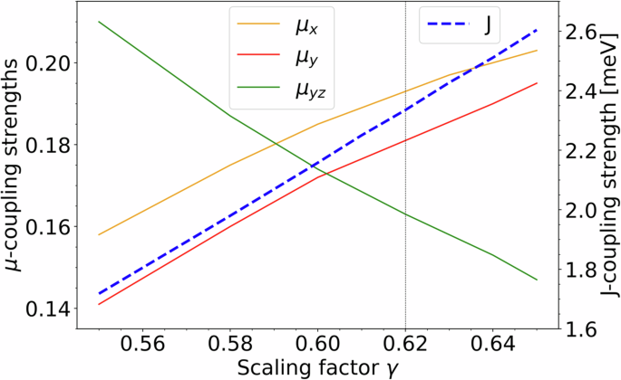
The magnetic couplings, as defined in Eq. (4), plotted against the nearest-neighbor Coulomb screening γ. The vertical dashed line at γ = 0.62 highlights our choice of the screening parameters for the final set of results.

Full size image

Thus, we find that when starting from an electronic Hamiltonian able to reproduce the main properties of the g-tensor, we are able to reconstruct the ferromagnetic Ising nature of the couplings and provide a relatively narrow microscopically compatible range for the smaller non-Ising terms, even when allowing γ to vary.

In Table 1 and 2 we display the calculated magnetic exchange parameters in the coordinate systems presented in Fig. 2a,b for a screening parameter γ = 0.62. This choice allows for a good reconstruction of the overall bandwidth of the measured excitation spectrum as shown in the next section. Table 1 and 2 also include the exchange interactions obtained in ref. ¹⁴ and ¹⁹ from fitting to experimental data. For this purpose, we transformed the notation in^14,19 into the coordinate systems used in this work.

Within the principal axis system (XYZ, see Table 2), following the fitted results, J is expected to be at ~ 2-2.5meV. While the Z-component exhibits the full influence of J, the X and Y-components are diminished by a significant amount. While ref. ¹⁴ predicts the S_XS_X and S_YS_Y components to be of similar magnitude at ~ 0.23J and ~ 0.27J, respectively, ref. ¹⁹ proposes a value of ~ 0.19J for the S_YS_Y component and no contribution at all from the S_XS_X component. Our data shows a trend similar to “Fit^INS”, though with slightly smaller values of μ_X and μ_Y and them lying closer to one another.

While our calculations predict small magnitudes for both μ_XY and μ_XZ, both fitting procedures set them to zero. Possibly, within the fitted models the effects of finite μ_XY and μ_XZ have been reabsorbed into an increased effective μ_YZ. Compared to our results, μ_YZ is indeed slightly larger in both experimental fittings. In conclusion, we observe that our calculated parameters have the strongest resemblance to those obtained in ref. ¹⁴.

Additional data was collected in Supplementary Table 2 to visualize the influence of the parameters in the Hubbard model on the couplings. Couplings resulting from Model^DFT and ({{{rm{Model}}}_{{rm{corr}}}}^{{rm{DFT}}}) as well as for γ = 0, 0.6 and 1 are presented. While μ_XY is very small in general, the orders of magnitude of μ_XZ and μ_YZ vary strongly with the underlying model parameters. μ_XZ changes depending on whether or not the adjustment to the crystal field is applied. Adding screening to the nearest-neighbor Coulomb interaction raises μ_YZ to values at the same level as the diagonal elements μ_X and μ_Y.

In Supplementary Table 3 a collection of magnetic couplings obtained through a selective choice of various contributions in the electronic Hamiltonian is presented. This allows for a deeper understanding of the influence of individual terms and the origin of different exchange terms. For example, the case of an ideal octahedral crystal field has been investigated. In that case, all anisotropies originating from the crystal field can be ruled out and other potential sources of anisotropic couplings can be uncovered. Similarly, as has been done before, by setting γ = 0 the ligand-mediated Hund’s exchange can be turned off while the exact influence of the kinetic exchange can be made visible by setting intersite hoppings to zero.

Based on the results the following conclusions can be made:

1. (i)

   In the absence of crystal field distortions the ligand-mediated Hund’s exchange exhibits ferromagnetic and nearly isotropic behaviour, while the kinetic exchange is antiferromagnetic and displays a significant anisotropy. However, large direct hoppings between d-orbitals on adjacent sites prevent the anisotropies from taking the Kitaev form (which arise primarily from ligand-mediated hoppings).

2. (ii)

   In the presence of the crystal field distortion, both, the kinetic and ligand-mediated Hund’s couplings are rendered anisotropic. Overall, the distorted crystal field now predominantly contributes to the anisotropy of the couplings by displaying dominant XXZ-type anisotropic behaviour of similar magnitude in both cases.

3. (iii)

   The final couplings emerge as a compromise of these contributions. The larger magnitude of the ferromagnetic ligand-mediated exchange term with respect to the antiferromagnetic hopping term leads to the overall ferromagnetic Ising character of the system.

4. (iv)

   The smaller μ_XY, μ_YZ and μ_XZ terms mostly originate from the kinetic exchange.

To benchmark our ab-initio procedure and the derived spin exchange model, we perform exact diagonalization calculations of the j_1/2 model in Eq. (4) and compare to INS¹⁴ and field-dependent THz spectroscopy data¹⁹. We therefore analyze the zero-temperature dynamical spin-structure factor

which we compute via the method of ref. ^47,48 using 150 Lanczos vectors for the spectral decomposition. Results for INS and THz data are presented in Figs. 4 and 5, respectively, both with a Gaussian broadening of σ = 0.028 meV. The weak inter-chain couplings leading to antiferromagnetic order between the chains are incorporated on a mean-field level through the addition of a simple term

to the Hamiltonian, for which we choose h_MF = 0.04 meV, oriented at the strength of mean-fields in previous studies^13,19. Within ED, we find in the γ = 0.62 model the ordered moment 〈g ⋅ S〉 to be within 1° off the Z-direction at B = 0, consistent with experiment^2,4,49,50.

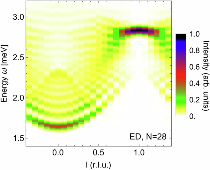
({{mathcal{S}}}^{XX}({bf{q}},omega )) for the exchange parameters given in Table 2 (γ = 0.62, Model({}_{{rm{corr}}}^{,text{DFT},})) at zero magnetic field computed via exact diagonalization on a periodic chain of N = 28 sites. The color map is chosen to match the experimental INS data plots in ref. ¹³.

Full size image

The dynamical response computed within ED of our first-principles derived exchange model (({{{rm{Model}}}_{{rm{corr}}}}^{{rm{DFT}}}) with γ=0.62) is in good agreement with the available experimental data^13,19. In particular, the zero-field INS response [Fig. 4] reproduces both the sharp high-energy mode near l = 1 and the broad scattering continuum away from l = 1¹³. The latter is induced by the off-diagonal non-Ising exchanges and can be understood as originating from a finite dispersion being lent to the domain-wall excitations^10,19. Near l = 0, the series of discrete bound states is reproduced¹³, which are induced by the longitudinal Weiss field from interchain coupling, that acts effectively as a confining potential for the domain wall excitations^6,17. The field-dependence seen in the THz spectrum [Fig. 5] is also qualitatively consistent with experiment¹⁹, featuring for the low-energy excitations a minimum of the excitation bandwidth near B = 2 T, for the medium-energy excitation a weaker B-dependence, and for the high-energy excitation a larger positive slope with field. Nevertheless, the relative intensities of the observed modes are not in perfect agreement with experiment¹⁹. Below, we discuss such quantitative deviations from the experiments in detail and provide arguments on their origin.

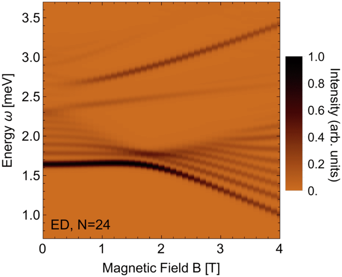
({{mathcal{S}}}^{XX}({bf{q}}=0,omega )) as a function of transverse magnetic field B (B∥b) for the exchange parameters given in Table 2 (γ = 0.62, ({{{rm{Model}}}_{{rm{corr}}}}^{{rm{DFT}}})) and g_Y = 3.13 from Table 3. Computed via exact diagonalization on a periodic chain of N = 24 sites. The color map is chosen to match the experimental THz data plots in ref. ¹⁹.

Full size image

The most prominent difference is the deviation in the overall energy scale which is slightly smaller in our ab-initio derived model compared to experiment. The peak visible in the INS spectrum displayed in Fig. 4 lies at approximately 2.85meV while the data in¹⁴ suggest an experimentally found energy of about 3.1meV for the peak. The THz spectrum is shifted equivalently. This energy scale is mainly incorporated in the size of the coupling J, which has a strong dependence on the screening of the nearest neighbor Coulomb terms. Smaller screening would increase J though this in turn would lead to the worsening of other aspects of the data. Other factors impacting J are also the magnitudes of the U_avg and J_avg Coulomb interactions on a single site. For our computation we used the parameters calculated in⁵¹ though also other values can be found in older literature, e.g. in⁵². Figure 5 also shows that the width of our energy distribution is smaller than in¹⁴. We found the size of the off-diagonal exchange couplings to be crucial for the width of the energy scale. Though larger off-diagonal contributions would have broadened the width of ω, this adjustment wasn’t possible within our framework.

Another noteworthy difference between our data and experiment is visible in the THz spectrum (see Fig. 5). Here the lowest lying energy mode has the strongest intensity which isn’t the case in the experimental findings in¹⁹. The intensity distribution could be adapted to the experimental THz spectrum through increasing off-site Coulomb screening though this would lower the energy scale further.

Summarizing, the INS and THz spectra extracted from our exact diagonalization approach of the first-principles modelled Hamiltonian are able to reproduce experimental findings on a qualitative and also partially on a quantitative level. We were also able to determine the microscopic origins to particular aspects of the spectra like nearest-neighbor Coulomb screening and on-site Coulomb interaction strengths. While we obtained an overall good qualitative agreement, note that we have not taken into account further neighbor exchanges, which are likely relevant for a further improved quantitative agreement¹³.

In this work, we have shown that the different refined models for the Ising spin-chain compound CoNb₂O₆ derived recently from experimental fitting^13,14,19,44 offer a mutually compatible view of the material that is consistent with microscopic considerations. Specifically, in this material, the local Co spins are strongly perturbed j_1/2 moments of the high-spin d⁷ configuration. The largest and most crucial contribution to the magnetic exchange is the ferromagnetic Goodenough-Kanamori (ligand-mediated) exchange involving the e_g electrons. This contribution acquires a bond-independent XXZ (Ising) anisotropy as a consequence of the strongly distorted CoO₆ octahedra, which also results in anisotropic g-tensors. The smaller bond-dependent couplings, the importance of which have been highlighted by the recent neutron and THz studies, arise as residual effects of d − d kinetic exchange processes involving the t_2g electrons. However, these residual terms do not follow precisely a Kitaev form because of the effects of the crystal field distortion, and the specific magnitudes of the d − d hoppings are more conducive to off-diagonal Γ couplings. These findings are all compatible with recent assertions about couplings between high-spin d⁷ compounds in³⁸, and offer significant insight into related Co²⁺ compounds currently under study in the context of bond-dependent magnetism.

In order to derive these conclusions, we have followed an ab-initio based approach that allows for a balanced treatment of the relevant contributions to the magnetic couplings, including the ligand-mediated ferromagnetic exchange, within a d-orbital picture. By adjusting the crystal field to match the experimental g − tensor, and varying the strength of the intersite Coulomb exchange, we have identified a relatively narrow range of magnetic Hamiltonians that can be considered microscopically compatible, and shown that they reproduce the experimentally observed rich dynamical response of the material. Specifically, for the bond-independent XXZ couplings, the two perpendicular (X, Y) contributions are smaller than the Ising (Z) coupling by a factor of roughly μ_X ≈ μ_Y ≈ 0.2. The largest bond-dependent coupling is of similar magnitude, and takes the form of off-diagonal μ_YZ. As pointed out in¹⁴, additional off-diagonal μ_XY and μ_XZ are also symmetry allowed, but were set to zero in both ref. ¹⁴ and ¹⁹ for simplicity. We find these couplings to be finite, but that they are the smallest terms in the Hamiltonian, partially justifying their omission in these previous studies. Overall, our derived couplings most closely resemble those of ref. ¹⁴, the main distinction being that ref. ¹⁴ employs μ_X = μ_Y, while ref. ¹⁹ employs μ_X = 0. Thus, while CoNb₂O₆ remains a very complex system to investigate within a purely ab-initio approach, the utilization of experimental input as guidance (such as the g-tensors and overall magnetic excitation bandwidth), allows for the elucidation of a microscopically consistent picture of the varied and competing exchange contributions. After many years of intensive research, the description of this paradigmatic material in quantum magnetism is finally coalescing, and continuing to hold new insights.

Structure and Symmetries

All calculations performed in this work are based on the crystal structure reported in ref. ⁴. CoNb₂O₆ crystallizes in the orthorhombic space group Pbcn featuring pseudospin 1/2 Co²⁺ zigzag chains extending along the crystallographic c-axis (Fig. 1). The magnetic Co²⁺ ions are linked through edge-sharing oxygen octahedra, forming chains characterized by alternating bonds. The neutron diffraction study in ref. ⁴ finds that the ground state magnetic structure below 1.97 K has the magnetic moments ordered ferromagnetically along the chains, with an antiferromagnetic pattern between chains. All Co octahedral environments are symmetry equivalent as follows. Nearest-neighbor Co sites along the chain are related by the c-glide indicated in Fig. 2a. The two chains per orthorhombic unit cell are symmetry-related by an n-glide (mirror in an ab plane passing through a Co site followed by translation by [1/2,1/2,0]), resulting in the presence of two distinct, but symmetry-related, easy axes^2,4,49,50.

In the discussion of the electronic Hamiltonian and magnetic couplings, it is useful to refer to two sets of coordinate systems. The “cubic” axes are defined as an orthonormal basis of vectors x, y and z, which point approximately along the octahedral Co-O bonds, as shown in Fig. 2a. They were obtained through symmetric (Löwdin’s) orthonormalization (see ref. ⁵³) from the direct Co-O bonds. In terms of the global crystallographic axes (a, b, c), these are:

In this coordinate system, the y-axis lies within the c-glide plane, which lies halfway between the x– and z-axes.

As is visible in Fig. 2a, one of the cubic axes is situated within the a–c plane with an angle of around ± 30° from the c-axis, where the sign of the angle alternates from chain to chain. Initial studies assumed that each easy axis would align with this cubic axis, leading to some disagreement in the literature (see^2,4,49,50) on that matter. As discussed below in further detail, we find that the direction of each easy axis lies in opposition to the corresponding cubic axis, meaning that for an angle of ± 30° for the cubic axis, the easy axis lies at ∓ 30° from the c-axis (see Fig. 2).

In order to enable comparisons between our results and those obtained experimentally in refs. ^14,19, we also refer to a coordinate system of “principal” axes denoted by uppercase letters X, Y and Z, where Z is aligned with the easy axis, as depicted in Fig. 2b. This coordinates are consistent with the definition in ref. ¹⁴.

With respect to (a, b, c), these “principal” axes are defined as:

where ϕ = + 30° is the canting angle. This definition sets the local Z-axis to be tilted by ϕ from the crystallographic c-axis in the negative a-direction. This choice of direction for Z is based on our estimates on the Ising axis orientation from determining the g-tensor. In this coordinate system, the Y-axis is perpendicular to the c-glide plane, while the X– and Z-axes lie within it.

Multi-Orbital Hubbard Model

In order to estimate the magnetic couplings, we apply an ab-initio based approach⁵⁴ (projED), which has been shown to yield reliable results for highly anisotropic spin Hamiltonians^48,55,56,57. The method is based on two steps. First, an electronic multi-orbital Hubbard Hamiltonian is obtained from a full-relativistic DFT calculation on the basis of appropriately constructed Wannier orbitals, as well as suitably defined Coulomb interactions. Second, the multi-orbital Hubbard Hamiltonian is exactly diagonalized on finite-size clusters. The eigenstates are then projected into the low-energy space. The resulting low-energy Hamiltonian in the orbital-basis is then projected onto an idealized space of pure j_1/2 doublets. The main contributions to these states are within the (t_2g)⁵(e_g)² subspace with seven electrons per site and J_eff = 1/2³⁸. The corresponding projection is defined in Supplementary Note 1.

We start with the description of all necessary terms contributing to the multi-orbital Hubbard Hamiltonian. The Hamiltonian in the basis of Co 3d-orbitals is given by:

The first term in Eq. (9) describes the hoppings between orbitals a and b on two Co-sites i and j where ({t}_{ij,sigma sigma {prime} }^{ab}) are the hopping integrals obtained from FPLO:

({{mathcal{H}}}_{{rm{nn-U}}}) describes the Coulomb interaction between different Co-ions i and j through the ligands. This is given by:

which resembles the typical intersite Coulomb term consisting of diagonal density-density contributions as well as a “Hund’s”-type coupling. Explicit inclusion of this latter term to the electronic Hamiltonian is crucial in order to account for ligand-centered exchange processes downfolded into the Co d-orbital basis. Especially the e_g-orbitals hybridize strongly with the ligands and produce large contributions to this term, which are manifestly important for correctly describing the magnetism of edge-sharing 3d materials (see, for example,⁵⁸). The terms ({tilde{U}}_{1}), ({tilde{U}}_{2}) and (tilde{J}) as well as the details of the derivation are discussed in the Intersite Coulomb Interactions section.

Finally, the last term in Eq. (9) includes all relevant on-site effects for each site i:

First, ({{mathcal{H}}}_{{rm{CF}}}) accounts for the crystal field splitting and ({{mathcal{H}}}_{{rm{SOC}}}) refers to spin-orbit coupling. The interaction term ({{mathcal{H}}}_{{rm{U}}}) includes all on-site contributions to the Coulomb interaction, which in its most general form is:

Here a, b, c and d label the d-orbitals while σ and (sigma {prime}) define the spin orientation. The U-matrix-elements are considered within the spherically symmetric approximation and are fully determined by the Slater integrals F₀, F₂ and F₄ via

Following ref. ⁵⁹, the ratio ({F}_{4}=frac{5}{8}{F}_{2}) is applied, which is a frequently used assumption for 3d orbitals. For the computations, the parameters U_avg = 5.1eV and J_avg = 0.9eV will be used, which have been obtained from constrained DFT calculations for CoO in ref. ⁵¹.

The material-specific contributions to the Hamiltonian contained in ({{mathcal{H}}}_{{rm{hop}}}), ({{mathcal{H}}}_{{rm{CF}}}), ({{mathcal{H}}}_{{rm{SOC}}}), and ({{mathcal{H}}}_{{rm{nn-U}}}) were estimated on the basis of DFT calculations. To that end, for ({{mathcal{H}}}_{{rm{hop}}}), and ({{mathcal{H}}}_{{rm{CF}}}+{{mathcal{H}}}_{{rm{SOC}}}) we perform a non-magnetic fully relativistic FPLO (see ref. ⁶⁰) calculation on a 12 × 12×12 grid within the generalized gradient approximation (GGA). Projective Wannier functions were used to obtain hopping parameters. The nearest-neighbor spin-diagonal hoppings can be found in Supplementary Note 2. The parametrization of the intersite Coulomb interactions is discussed below. We first refine the crystal field in order to ensure consistency with the measured g-tensors.

Crystal Field Splitting and g-Tensor

In this section, we first discuss the modelling of the local crystal field, and its consequences on the g-tensor.

In Co 3d⁷ compounds, the relative weakness of the SOC effectively enhances the sensitivity of the low-energy spin interactions and g-tensor to crystal-field distortions, which influence the specific spin-orbital composition of the local moments. As a consequence, accurate modelling of the local single-ion state is a prerequisite for understanding the intersite exchange couplings. As demonstrated in ref. ⁶¹, Wannier fitting only sometimes achieves the necessary accuracy to reproduce the experimental crystal field energies. We therefore introduce some parameter adjustments in our electronic Hamiltonian to ensure consistency with the experimentally determined g-tensor. Experimentally, the g-tensor has been estimated in various works. Ref. ¹² fitted g-tensor principal values and orientations from EPR and INS spectra for two different samples. They find two of the g-values to be relatively close to another, and a much larger third g-value, where the principal axes are in agreement with the definition in Eq. (8) for an angle ϕ = 37°. Ref. ¹⁴ presents similar data on the principle values. The comparison of our results to the g-tensor proposed in ref. ¹⁴, which assumed that the principal axes were along the XYZ-axes (ϕ = 30°), is visible in Table 3.

In order to compute the g-tensor from first principles, we diagonalize the on-site Hamiltonian Eq. (12) with an additional term ({{mathcal{H}}}_{{rm{Zeeman}}}) that describes the coupling of the angular momentum (overrightarrow{L}) and spin (overrightarrow{S}) of the Co-ions to an external magnetic field (overrightarrow{B}):

After projecting the resulting low-energy (2 × 2) Hamiltonian onto ideal j_1/2 states, the g-tensor is obtained by taking numerical derivatives with respect to different components of (overrightarrow{B}). Due to a 2-fold rotation axis parallel to the crystallographic b-axis going through each Co site, one of the principal axes of the g-tensor is enforced to be parallel to the b-axis (coincident with the Y-axis).

As a starting point for discussion, we first consider the crystal field splitting matrix ({{mathbb{M}}}_{{bf{CF}}}) obtained directly from the DFT calculation after Wannierization. Written in terms of orbitals d_xy, d_yz, d_xz, ({d}_{{z}^{2}}) and ({d}_{{x}^{2}-{y}^{2}}), this is (in meV):

where for readability these values were gauged such that ({{mathbb{M}}}_{xy,xy}={{mathbb{M}}}_{yz,yz}=0). Performing the calculation for the g-tensor starting from ({{mathbb{M}}}_{{bf{CF}}}^{{rm{DFT}}}) yields principal axes of the g-tensor corresponding to X, Y, Z of Eq. (8), but with an incorrect canting angle of ϕ ≈ 45° (complete g-tensor given in Supplementary Note 4, instead of ϕ ≈ 30° from experiment^4,14. Since the magnetic couplings depend strongly on the crystal field, ({{mathbb{M}}}_{{bf{CF}}}) does not represent an adequate starting point for further calculations.

After investigating the effects of various alterations to ({{mathbb{M}}}_{{bf{CF}}}^{{rm{DFT}}}), we conclude that this discrepancy is likely due to an overestimation of the splitting between the xy/yz-orbitals and the xz-orbital. Such a discrepancy can arise in various ways. First, we rely on the accuracy of the starting structure; small changes in the atomic positions can lead to significant effects on the computed CFS matrix. Second, inherent to the Wannier interpolation in DFT is an effective inclusion of the mean-field Coulomb terms into the single-particle Hamiltonian. In relatively undistorted local environments, these mean-field contributions to the orbital energies can be expected to be relatively orbital-independent within the d-orbitals, i.e. provide only a constant diagonal shift of the orbital energies. However, with lower symmetry environments, the mean-field contributions may instead display significant orbital-dependence. It is therefore more appropriate to improve the crystal field estimates by fitting to available experimental data, whenever possible.

In the present case, we find that the minimal modification of ({{mathbb{M}}}_{{bf{CF}}}^{{rm{DFT}}}) required to reflect the major aspects of the experimental g-tensor (see refs. ^4,12) is simply to set ({{mathbb{M}}}_{xz,xz}) in Eq. (16) to 15meV, i.e. reducing the t_2g splitting. This results in principal axes of the g-tensor that correspond to a canting of ϕ ≈ 30. 8° in Eq. (8), and yields the principal g-values shown in Table 3 under “({{{rm{Model}}}_{{rm{corr}}}}^{{rm{DFT}}})” (complete g-tensor is given in Supplementary Note 4). The modification of the crystal field reduces the previously large difference between g_X and g_Y (see Supplementary Note 4), and reproduces the large anisotropy of the g_X/g_Y and g_Z principal values. Altogether, the comparison to experimentally fitted g-values of ref. ¹⁴ (“Fit^INS” in Table 3) yields a very good agreement.

From now on, we perform all calculations of the intersite couplings employing ({{rm{Model}}}_{{rm{corr}}}^{{rm{DFT}}}) that includes the corrected crystal field splitting, setting ({{mathbb{M}}}_{xz,xz}) in Eq. (16) to 15meV.

Intersite Coulomb Interactions

The nearest-neighbor magnetic interactions between edge-sharing octahedra of high-spin Co²⁺ ions are strongly influenced by ferromagnetic Coulomb exchange interactions through the ligands³⁸, similar as for other 3d ions⁵⁸. In the standard picture of these contributions considering explicitly the metal d and ligand p orbitals, the ferromagnetic contribution arises at order ({J}_{H}^{p}{t}_{pd}^{4}/{Delta }_{pd}^{4}), where ({J}_{H}^{p}) refers to the Hund’s coupling of the ligands, t_pd is the hopping between the p and d orbitals, and Δ_pd is the charge transfer energy. These are discussed as “charge-transfer” processes in ref. ²⁴. They capture the effect that two holes, nominally associated with different sites, may meet on the same ligand, and experience Hund’s coupling that reduces the energy of the triplet configuration (see Fig. 6). When projected into the basis of d Wannier functions, this term is reinterpreted as an effective intersite Coulomb interaction. The weight of the p-orbitals in these Wannier functions scale like ({({t}_{pd}/{Delta }_{pd})}^{2}). As a consequence of the fact that the d-orbital Wannier functions of different Co sites have finite coefficients on the same ligand, rotation of the ligand Coulomb interactions into the Wannier basis results in intersite Coulomb interactions of order ({J}_{H}^{p}{t}_{pd}^{4}/{Delta }_{pd}^{4}).

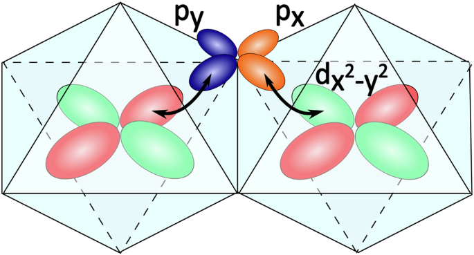
Two neighboring octahedra with Co-atoms at each center. The hybridization of their e_g-orbitals with ligand p-orbitals leads to an effective intersite Coulomb repulsion when holes interacting at the ligand repel each other. Here the process is visualized for ({d}_{{x}^{2}-{y}^{2}}) orbitals.

Full size image

To make this qualitative discussion concrete and to arrive at the interaction ({{mathcal{H}}}_{{rm{nn-U}}}) summarized in Eq. (11), one can write the creation operators associated with the bare p-orbitals α on ligand atom n in terms of p-orbital Wannier functions located at the same site, and d-orbital Wannier functions a on Co site i through:

where the tilde indicates mixed p/d Wannier orbitals. ϕ_nασ and ({phi }_{ia}^{nalpha }) represent the overlap between Wannier functions. The corresponding values can be obtained from FPLO. The latter term shows how the oxygen p-orbitals can be expressed via the wavefunction overlap with cobalt d-orbitals. In the downfolded basis, only the (tilde{d}) Wannier orbitals are explicitly considered. The bare Coulomb interaction for the p-orbitals, as it is given for p-orbitals in⁶², is:

with

Inserting the ansatz in Eq. (17) into Eq. (18), and retaining those terms with all d-orbital operators leads to the expression shown in Eq. (11), for which the coupling matrices ({tilde{U}}_{1}), ({tilde{U}}_{2}) and (tilde{J}) are defined as:

Here, ({A}_{ab}equiv gamma {sum }_{n,alpha ne beta }| {phi }_{ia}^{nalpha }{| }^{2}| {phi }_{jb}^{nbeta }{| }^{2}), ({B}_{ab}equiv gamma {sum }_{n,alpha ne beta }{phi }_{ia}^{nalpha }{phi }_{ia}^{nbeta }{phi }_{jb}^{nalpha }{phi }_{jb}^{nbeta }) and ({C}_{ab}equiv gamma {sum }_{n,alpha }| {phi }_{ia}^{nalpha }{| }^{2}| {phi }_{jb}^{nalpha }{| }^{2}).

({J}_{H}=frac{4}{25}{F}_{2}^{p}) refers to the Hund’s exchange energy associated with the O 2p orbitals and ({F}_{2}^{p}) to the according Slater integral. Following ref. ⁶³, ({F}_{2}^{p}) for oxygen p-orbitals is expected to lie at 6eV. U₀ corresponds to ({F}_{0}^{p}+frac{4}{3}{J}_{H}). For our calculations we use J_H = 0.3U₀ in analogy to ref. ²⁴, and estimate A_ab, B_ab, and C_ab from non-relativistic FPLO calculations. Finally, we introduced a scaling factor γ to the overlap integrals, in order to account for screening of the Coulomb interactions with respect to the bare Slater integral.

The nearest-neighbor Coulomb interactions influence the magnetic exchange primarily through the (tilde{J})-terms, which result in a ferromagnetic interaction when projected into the j_1/2 basis. The ({tilde{U}}_{1}) and ({tilde{U}}_{2}) represent spin-independent density-density interactions, and have little influence on the magnetic couplings (see Supplementary Note 4 for comparison). The obtained (tilde{J}) matrix on bond 2 (see Fig. 2b), in terms of d_xy, d_yz, d_xz, ({d}_{{z}^{2}}) and ({d}_{{x}^{2}-{y}^{2}}), is (({tilde{U}}_{1}) and ({tilde{U}}_{2}) are given in Supplementary Note 2):

The dominant contributions to intersite coupling (in all of ({tilde{U}}_{1}), ({tilde{U}}_{2}), (tilde{J})) stem from the e_g-orbitals, due to their much larger hybridization with the ligand p-orbitals. As discussed in^24,26,38, it is the presence of the e_g electrons in the high-spin d⁷ configuration that leads to a significant effect of the ferromagnetic ligand exchange processes.