Universal relations and bounds for fluctuations in quasistatic small heat engines
Introduction
Formidable advances in physics and nanotechnology have led to the construction of miniaturized heat engines of the size of a colloidal particle1,2,3,4,5,6,7 or even smaller8,9,10,11,12,13,14. Such microscopic heat engines constitute a perfect target study for understanding the double-sided challenges of miniaturization. On the one side, there is the aim of understanding the fundamental thermodynamic principles of small machines15,16,17,18,19,20,21; on the other side, there is the pursuit of the optimal design of artificial devices6,18,22,23,24. The relevance of fluctuations in thermodynamic quantities of small machines, such as work, heat, or entropy has been predicted by the theoretical framework of stochastic thermodynamics25,26,27,28,29,30,31,32,33,34 and reported in numerous experimental realizations of mesoscopic heat engines with tremendous accuracy2,4,5,35. As demonstrated by the experiment of ref. 4, for instance, fluctuations of thermodynamic quantities can be dominant over their average values. Such theoretical and experimental progress highlighted the need to characterize small machines’ fluctuations through higher moments of their thermodynamic quantities beyond their mean values36,37,38,39,40,41,42,43,44,45,46,47,48. Although Carnot’s celebrated result regarding the ratio between average work and heat of cycles has been known for a long time, there is still no universal bound on the fluctuations of work and heat, even for quasistatic cycles.
In this article, we develop a theory that describes the (n ≥ 2)th-order moments of the work and heat of small heat engines that are subject to thermal fluctuations and test our predictions with experimental data from the Brownian Carnot engine35, a Carnot engine with a Brownian particle as its working substance. In particular, we analyze the statistical properties of reversible Carnot cycles through moments of arbitrary order, finding that they show universal features in the line of Carnot’s classical result: with exclusive dependence on the temperature ratio Tc/Th between the hot (Th) and cold (Tc) heat baths. Furthermore, we show that the ratio between the fluctuations of work and heat for the Carnot cycle provides a universal upper bound for this quantity among cycles operating between the temperatures Th and Tc consisting of quasistatic strokes. Our analytical results are tested using previous experimental data of the Brownian Carnot engine35, exploring their validity from the quasistatic limit to the non-equilibrium performance in the non-quasistatic regime. Our results pave the way to designing reliable microscopic heat engines by reducing the fluctuations of the work output without lowering the average work and efficiency.
Results
Working substance
Systems with a small number of degrees of freedom do not necessarily relax into an equilibrium state during adiabatic processes even if they are quasistatic (Throughout the present paper, the word “adiabatic” means that there is no energy exchange between the system and environment in the form of heat.). For example, systems with more than two discrete energy levels initially in equilibrium at some temperature are no longer at equilibrium for any temperature after the energy of one of the levels is changed quasistatically. Therefore, in establishing thermal contact with a heat bath after an adiabatic process, an irreversible change in the energy distribution occurs if the final state of the adiabatic process does not follow the canonical distribution at the temperature of the bath16. To realize the reversible Carnot cycle with a small system, an extra condition is required to avoid such irreversibility, which does not exist for macroscopic systems. In the present work, we consider a class of working substances that allows us to implement the desired cycle free from this irreversibility for arbitrary values of Th and Tc. For the experimental platform to realize our setup, systems with high controllability and high (and controllable) isolation from the environment, such as trapped ions49 and levitated nanoparticles50,51 are promising.
Suppose a system is in thermal equilibrium at temperature T1 with an external control parameter λ at λ1. Then, a quasistatic adiabatic process is performed by slowly changing λ from λ1 to λ2. After the quasistatic adiabatic process, the system is put in contact with a thermal bath at temperature T2. The internal energy of the initial and final state of the adiabatic process is denoted by E1 and E2, respectively. At the beginning of the quasistatic adiabatic process, the system is in a microstate Γ1 in the phase space with energy ({E}_{1}={H}_{{lambda }_{1}}({Gamma }_{1})) whose distribution is given by the canonical ensemble for ({H}_{{lambda }_{1}}) at T1. During the quasistatic adiabatic process, the system evolves deterministically by Hamilton’s equations of motion, and the internal energy of the system changes following the adiabatic theorem such that the phase space volume Iλ(E) enclosed by the iso-energy surface at E (the so-called number of states) is invariant under the slow change of λ. Here, ({I}_{lambda }(E)equiv int,theta left(E-{H}_{lambda }(Gamma )right),{d}Gamma) with θ being the Heaviside step function. To ensure reversibility, the energy distribution before and after the thermal contact should be the same, so
up to a constant for any realization [adiabatic-reversibility (AR) condition]16,52. In order to guarantee that we can find an appropriate final parameter λ2 that fulfills the AR condition, the initial and final energies of the quasistatic adiabatic process need to be linked by E1 = ϕ(λ1, λ2)E2 with a function ϕ(λ1, λ2) that solely depends on the initial and final parameter values λ1 and λ252.
To implement the reversible Carnot cycle for any choice of the baths’ temperatures and the parameter λ at the starting (or ending) point of the adiabatic strokes, the AR condition has to be satisfied for arbitrary values of T1, T2, and λ1 (or λ2). Hence, the working substance should satisfy the above relation, E1 = ϕ(λ1, λ2)E2, with ϕ(λ1, λ2) such that for every fixed λ1 = λ, the function gλ(λ2) ≡ ϕ(λ, λ2) of λ2 can take any value of T1/T2. It is noted that the typical working substance for microscopic heat engines falls in this class of working substance. For example, a single particle trapped in a harmonic oscillator potential with controllable spring constant, which is commonly employed in most of the experiments so far2,4,5,7,35, and a single particle trapped in a box potential with controllable box width are the cases since their number of states is in the form of Iλ(E) = f(λ) Eα with a positive unbounded function f. This holds, e.g., for a scale-invariant potential Vλ(x) satisfying Vλ(ax) = ∣a∣b Vλ(x) with positive real constant b > 0, where a is the scaling factor and x represents the position of the particle.
Universal relations between work and heat fluctuations of the Carnot cycle
All relevant quantities of a microscopic heat engine are stochastic by nature, and therefore they fluctuate over different realizations of a given protocol. When averaged over many realizations of a given protocol, the mean values of work and heat converge, and their stochastic nature is revealed by their probability distributions (Fig. 1b).
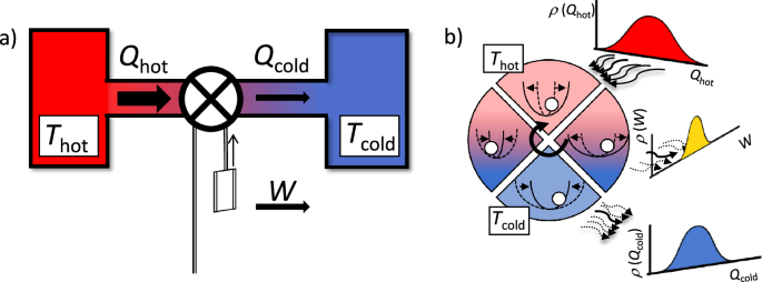
a Carnot’s theorem bounds the maximum work that can be extracted from two thermal baths based on the ratio between the hot and cold temperatures. b When the heat engine is miniaturized, see standard protocol depicted between the hot bath (up, red) and the cold one (down, blue) with the four processes sketched, thermal fluctuations become significant, making all the energy fluxes stochastic, described by their probability density functions. Our results show that the various moments of the energetics also scale with the temperature ratio.
In many stochastic systems, mean values are not good quantities to characterize their behavior, but the moments of their distributions need to be accounted for. It is indeed the case for the experiments of the Brownian heat engines, where the fluctuations of thermodynamic quantities are comparable to their mean values2,4. The nth order central moment (leftlangle {(Delta X)}^{n}rightrangle) of a random variable X is defined as (leftlangle {(Delta X)}^{n}rightrangle equiv leftlangle {(X-leftlangle Xrightrangle )}^{n}rightrangle), where (leftlangle Xrightrangle) and (Delta Xequiv X-leftlangle Xrightrangle) are the statistical average and the fluctuation of “X”, respectively. As we detail in the subsection of “Derivation of Eqs. (1), (2), and (4)” in the “Methods” section, one can derive a neat relation between the higher-order statistics of the work output W and the heat input Qh for the reversible Carnot cycle:
which holds for any integer n ≥ 2. Here, Th and Tc are the temperatures of the hot and cold heat baths, respectively, and ηC ≡ 1−(Tc/Th) is the Carnot efficiency. This formula relates any higher-order statistics of work output and heat input such as variances for n = 2, skewness for n = 3, kurtosis for n = 4, and so forth. Equation (1) is one of the main results of this work. It is noted that the ratio η(n) for the Carnot cycle given by Eq. (1) shows the universal form which depends only on the ratio Tc/Th. As we will demonstrate later, our relation (1) is more useful to control each higher-order statistic of W compared to the stochastic efficiency (hat{eta }equiv W/{Q}_{{{rm{h}}}}) since Eq. (1) contains only the central moments of W and Qh of the same order. The relation (1) is obtained from the AR condition and from the fact that the fluctuations of work through quasistatic isothermal strokes are negligible: the fluctuations of work output Wisoth through the isothermal stroke vanish in the limit of long duration τ of the stroke as (Delta {W}_{{{rm{isoth}}}}={W}_{{{rm{isoth}}}}-leftlangle {W}_{{{rm{isoth}}}}rightrangle =O({tau }^{-1/2}))16,53 (see also the subsection “Fluctuations of work and heat in the quasistatic isothermal process” in the “Methods” section for details).
The second relation that we have obtained (see the subsection “Derivation of Eqs. (1), (2), and (4)” in the “Methods” section for details of the derivation) connects the central moments of the heat exchanged with the heat baths and their temperatures:
for any integer n ≥ 2. It is noted that this relation is analogous to the “central relation of thermodynamics” called by Feynman54, (leftlangle {Q}_{{{rm{h}}}}rightrangle /{T}_{{{rm{h}}}}=leftlangle {Q}_{{{rm{c}}}}rightrangle /{T}_{{{rm{c}}}}), which holds between the two isothermal strokes in the reversible Carnot cycle. Since the temperatures Tc and Th are arbitrary, these relations hold for two arbitrary quasistatic isotherms connected by two quasistatic adiabats. Finally, the variance of work and the sum ΔQ(2) of the heat fluctuations over the separated sequences of heat-exchanging strokes, given by
satisfy another universal relation depending solely on the ratio Tc/Th:
Here, we remark that the same relation as Eq. (1) could also be derived from the integral fluctuation theorem55,56. As discussed in detail in the subsection “Integral fluctuation theorems and ({eta }_{{{rm{C}}}}^{(n)})” of the “Methods” section, we could obtain W = [1−(Tc/Th)]Qh from the integral fluctuation theorem for a cyclic protocol starting from the equilibrium state at Tc. Similarly, for a protocol starting from the equilibrium state at Th, we obtain W = [(Th/Tc)−1]Qc. However, it is noted that the random variables in the above two equations obtained from the fluctuation theorems for different initial points should be regarded as different random variables (even for W in these equations), which belong to different ensembles. Obviously, the fluctuation ΔE of the internal energy change through one cycle, E = (Qh−Qc)−W, depends on the temperature of the initial point, so that work and heat for different protocols with different initial points are different random variables. Therefore, it is not trivial to derive the relations given by Eqs. (2) and (4) by combining the above two equations obtained for different initial points, and also not trivial to prove W = [1−(Tc/Th)]Qh for an initial state other than the equilibrium state at Tc from the integral fluctuation theorems. While it is hard to discuss W, Qh, and Qc for the same protocol in the derivation based on the integral fluctuation theorems, our bottom-up approach employed in the subsection “Derivation of Eqs. (1), (2), and (4)” in the “Methods” section can handle all the random variables of W, Qh, and Qc for the same protocol at the same time, and allows us to deal with the effects of the endpoints more carefully, which are important in the discussion of the fluctuations for a single cycle. In addition, for our bottom-up approach, deriving the relations (1), (2), and (4) for any other initial point is straightforward. Because of the above reasons, we took the bottom-up approach in our derivation provided in the subsection “Derivation of Eqs. (1), (2), and (4)” in the “Methods” section.
Universal bounds on η
(2) and ξ
(2)
Next, we show that the ratios ({eta }^{(2)}equiv leftlangle Delta {W}^{2}rightrangle /leftlangle Delta {Q}_{{{rm{h}}}}^{2}rightrangle) and ({xi }^{(2)}equiv leftlangle Delta {W}^{2}rightrangle /Delta {Q}^{(2)}) for the Carnot cycle, given by Eqs. (1) and (4), provide upper bounds for these ratios among general quasistatic cycles using the considered working substance. (More precisely, the bound on ξ(2) will be shown for an arbitrary quasistatic cycle, and the bound on η(2) will be shown for a large class of quasistatic cycles, which include most of the typical cycles.) We consider cycles consisting of any of the quasistatic isothermal, quasistatic adiabatic, isochoric, or quasistatic isobaric strokes operating between the temperatures Tc and Th (see Fig. 2).
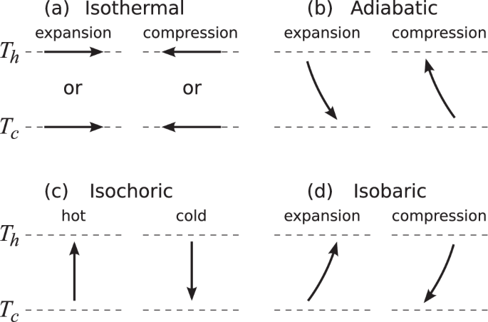
Four types of processes (a quasistatic isothermal, b quasistatic adiabatic, c isochoric, and d quasistatic isobaric strokes) are shown on the T−λ plane, where the T-axis is in the vertical direction, and λ-axis is in the horizontal direction. Here, figures show the case in which λ is chosen such that the increase (decrease) of λ corresponds to the increase (decrease) of the volume of the system (e.g., the width of a box potential or the inverse of the spring constant of a harmonic oscillator potential is taken as λ). For another choice of λ where the increase (decrease) of λ corresponds to a decrease (increase) of the volume and the horizontal axis of the figure should be λ−1-axis.
Isobaric processes are those during which the generalized pressure (Pequiv -leftlangle partial {H}_{lambda }/partial lambda rightrangle) is constant. Here, the change of P due to the variation of λ should be compensated by that due to the heat exchange between the working substance and the heat bath. Since the system is in contact with a heat bath during the isobaric stroke, work fluctuations of the quasistatic isobaric stroke are negligible due to the same reason as the isothermal stroke. As an example, let us choose λ such that the increase of λ corresponds to the increase of the volume. By expanding the volume (or λ), the working substance does work. Therefore, the internal energy is used by this expansion, and the pressure of the working substance usually decreases unless there is energy input from the bath. Thus, the heat input should be positive to keep P constant, so that the temperature of the working substance increases. Consequently, a quasistatic isobaric stroke is shown by an upward-sloping curve on the T−λ plane for such a choice of λ (Fig. 2d).
To perform quasistatic isobaric processes, we surround the working substance with a “quasi-adiabatic wall”, which is made of an imperfect heat insulator. When we make a thermal contact between the working substance and the heat bath, heat conduction between them and the thermalization of the working substance occur simultaneously. By surrounding the working substance with the quasi-adiabatic wall and making thermal contact with a heat bath through this wall, we can make the timescale of the heat conduction much larger than that of the thermalization. In this situation, the working substance is thermalized at every moment, i.e., it is always in a canonical state, even if there is an infinitesimally small but continuous heat flux between the working substance and the heat bath that lasts until the temperature of the former reaches that of the latter. Then, quasistatic isobaric processes can be performed by changing λ with keeping P constant, which is given by the canonical average of −∂Hλ/∂λ for instantaneous values of the parameter λ and the temperature T of the working substance. For example, for a working substance with Iλ(E) = f(λ)Eα, the generalized pressure is given by P = kBTf(λ)−1∂λ f(λ), where kB is the Boltzmann constant, and the instantaneous values of λ and T are related to keeping P fixed at the initial value. In the typical experimental platforms of thermodynamics of small systems, such timescale separation between thermalization in the working substance and heat conduction between the working substance and a bath could be possible for a particle trapped in a harmonic oscillator potential coupled to a thermal environment. The phase space distribution function of this system is always Gaussian provided the initial distribution function is Gaussian. Since the Gaussian phase space distribution function in this system can be identified as a canonical state with some effective temperature Teff, the system can be regarded as if it is always in thermal equilibrium at an instantaneous value of Teff at every moment even if Teff is different from the temperature of the bath. On the other hand, the timescale for the heat exchange between the system and bath is determined by the mobility (or diffusion coefficient) of the particle. Thus, by setting the mobility sufficiently small, we could realize the above-mentioned timescale separation.
Isochoric processes are those during which λ is fixed, and heat is exchanged between the working substance and the heat bath. Since λ is fixed through the isochoric stroke, work output, and work fluctuations are zero. On the T−λ plane, an isochoric stroke with the hot (cold) heat bath is shown by an upward (downward) vertical line (Fig. 2c). If we make direct thermal contact between the working substance and the heat bath, the final state of the isochoric process is a canonical state at the temperature of the bath; however, if we make a thermal contact through the quasi-adiabatic wall, the temperature of the final canonical state can be any value between the initial state and the temperature of the bath.
Now we consider the fluctuations of work output and heat input through the above four kinds of processes. Suppose the initial and the final points of the stroke are points i and i + 1, and the variances of work output and heat input through the stroke i → i + 1 are denoted by (leftlangle Delta {W}_{ito i+1}^{2}rightrangle) and (leftlangle Delta {Q}_{ito i+1}^{2}rightrangle), respectively. Regarding the heat exchanging strokes (i.e., quasistatic isothermal, isochoric, and isobaric strokes), since the work fluctuations ΔWi→i+1 are negligible and the internal energies Ei and Ei+1 at their endpoints i and i + 1 are independent, heat fluctuations of these strokes are given by (leftlangle Delta {Q}_{ito i+1}^{2}rightrangle =leftlangle Delta {E}_{i+1}^{2}rightrangle +leftlangle Delta {E}_{i}^{2}rightrangle). For quasistatic adiabatic strokes, since Wi→i+1 = Ei−Ei+1 = [1−(Ti+1/Ti)]Ei = [(Ti/Ti+1)−1]Ei+1 using the AR condition (Ei/Ti = Ei+1/Ti+1) for the third equality, the work fluctuations are given by (leftlangle Delta {W}_{ito i+1}^{2}rightrangle ={[1-({T}_{i+1}/{T}_{i})]}^{2}leftlangle Delta {E}_{i}^{2}rightrangle ={[({T}_{i}/{T}_{i+1})-1]}^{2}leftlangle Delta {E}_{i+1}^{2}rightrangle). The results of (leftlangle Delta {W}_{ito i+1}^{2}rightrangle) and (leftlangle Delta {Q}_{ito i+1}^{2}rightrangle) for each type of process are summarized in Table 1.
Suppose we have an arbitrary cycle consisting of any sequence of the above four types of processes operating between the bath temperatures Tc and Th. For the clarity of the discussion, we choose the starting point such that the final stroke is an adiabatic one. In the case of cycles with no adiabatic strokes, trivially (leftlangle Delta {W}^{2}rightrangle =0) and thus ξ(2) = η(2) = 0. Among all the N nodes (k = 0, 1, 2, ⋯ , N) of the cycle with points 0 and N being identical, we consider their subsets of both ends of quasistatic adiabatic expansion and compression strokes. For the ith adiabatic expansion (compression) stroke, the initial and the final points are denoted by Ji and Ji + 1 (Ki and Ki + 1), and the energy and the temperature of these points satisfy the AR condition reading ({E}_{{J}_{i}+1}=({T}_{{J}_{i}+1}/{T}_{{J}_{i}}),{E}_{{J}_{i}}) [({E}_{{K}_{i}}=({T}_{{K}_{i}}/{T}_{{K}_{i}+1}),{E}_{{K}_{i}+1})]. Since only the adiabatic strokes yield work fluctuations, fluctuation of total work output through the cycle is given by
Regarding the sum of the heat fluctuations ΔQ(2), the endpoints of the adiabatic strokes must be connected to the other kinds of strokes, and only these endpoints of the adiabatic strokes contribute to ΔQ(2). On the other hand, if there are heat-exchanging strokes (those other than quasistatic adiabatic strokes) consecutively, the node connecting them does not contribute to ΔQ(2) because the internal energies at the final point of the preceding stroke and at the initial point of the following one cancel each other. Thus,
Since the temperatures ({T}_{{J}_{i}}) and ({T}_{{J}_{i}+1}) (({T}_{{K}_{j}}) and ({T}_{{K}_{j}+1})) are in the region of [Tc,Th] and ({T}_{{J}_{i}}ge {T}_{{J}_{i}+1}) (({T}_{{K}_{j}+1}ge {T}_{{K}_{j}})), from Eqs. (5) and (6) we obtain (see the subsection “Derivation of Eqs. (7) and (8)” in the “Methods” section for details)
Thus, for the ratio ({xi }^{(2)}equiv leftlangle Delta {W}^{2}rightrangle /Delta {Q}^{(2)}), we finally obtain
where ({xi }_{{{rm{C}}}}^{(2)}equiv {[1-({T}_{{{rm{c}}}}/{T}_{{{rm{h}}}})]}^{2}/[1+{({T}_{{{rm{c}}}}/{T}_{{{rm{h}}}})}^{2}]) is the ratio ξ(2) for the Carnot cycle given by Eq. (4). Since a sum of the fluctuations of heat inputs for each stroke trivially satisfies ({sum }_{i = 0}^{N-1}leftlangle Delta {Q}_{ito i+1}^{2}rightrangle ge Delta {Q}^{(2)}), another ratio ({tilde{xi }}^{(2)}equiv leftlangle Delta {W}^{2}rightrangle /mathop{sum }_{i = 0}^{N-1}leftlangle Delta {Q}_{ito i+1}^{2}rightrangle) defined with this quantity is also bounded by (xi_{rm C}^{(2)}): ({tilde{xi }}^{(2)}le {xi }^{(2)}le {xi }_{{{rm{C}}}}^{(2)}). Note that ({tilde{xi }}^{(2)}={xi }^{(2)}) for the Carnot cycle.
Regarding the ratio ({eta }^{(2)}equiv leftlangle Delta {W}^{2}rightrangle /leftlangle Delta {Q}_{{{rm{h}}}}^{2}rightrangle), the value ({eta }_{{{rm{C}}}}^{(2)}) for the Carnot cycle gives the maximum value among any cycle in which quasistatic adiabatic expansion (compression) strokes are preceded (followed) by a stroke with the hot bath (if it is not the case, it is possible to have ({eta }^{(2)} , > , {eta }_{{{rm{C}}}}^{(2)}), see Supplementary Note 1 for an example). This is a natural condition since the thermal energy needs to be taken from (dumped to) a heat bath before the adiabatic expansion (compression). Indeed, most of the typical cycles, including the Otto, Brayton, Stirling, and Ericsson cycles, satisfy this condition. In such cycles, the energy fluctuations at the initial point Ji (final point Kj + 1) of all the quasistatic adiabatic expansion (compression) strokes contribute to (leftlangle Delta {Q}_{{{rm{h}}}}^{2}rightrangle). Thus,
From Eqs. (7) and (10), we get
where ({eta }_{{{rm{C}}}}^{(2)},, (={eta }_{{{rm{C}}}}^{2})) is the ratio η(2) for the Carnot cycle given by Eq. (1) for n = 2. For the Stirling and Ericsson cycles, (leftlangle Delta {W}^{2}rightrangle =0) and thus η(2) = 0. For the Otto and the Brayton cycles, taking the working substance with Iλ(E) = f(λ) Eα as an example, we get ({eta }^{(2)}={[1-({T}_{2}/{T}_{1})]}^{2}), where T1 and T2 are the initial and the final temperatures of the quasistatic adiabatic expansion stroke. Since 1 ≥ T2/T1 ≥ Tc/Th, this η(2) indeed satisfies ({eta }^{(2)}le {eta }_{{{rm{C}}}}^{(2)}). Finally, we remark that, besides the Carnot cycle, there also exist other cycles that give the same value of ({eta }^{(2)}={eta }_{{{rm{C}}}}^{(2)}) and ({xi }^{(2)}={xi }_{{{rm{C}}}}^{(2)}) (see Supplementary Note 2).
Experimental verification
Next, we compare our theoretical results against our previous experiment of the Carnot engine using an optically trapped Brownian particle (the so-called Brownian Carnot engine)4, which is a typical setup for microscopic heat engines. Differences to keep in mind between the Brownian Carnot engine and the true Carnot cycle considered in our work are the following: (1) The working substance of the Brownian engine is always in contact with a thermal environment whose temperature is continuously controllable. (2) The protocol of the Brownian Carnot engine involves two isothermal strokes and two isentropic strokes (i.e., those during which the Shannon entropy of the working substance is constant35) instead of the isolated adiabatic strokes considered in the present work. Since the working substance of the Brownian heat engine is always in contact with a bath, the variance of work is zero, so that η(2) = 0 in the quasistatic limit. Nevertheless, there is a correspondence relation between the work distribution of the isolated adiabatic process and the heat distribution of the isentropic strokes for the Brownian Carnot engine in the quasistatic limit (see the subsection “Comparison with experimental data” in the “Methods” section for details of the correspondence relation). Therefore, through this correspondence relation, we can simulate the fluctuations of work and heat of the quasistatic Carnot cycle from the experimental data of the Brownian Carnot engine by assuming that the Brownian particle is near equilibrium.
Since the relaxation time (~0.1 μs) of the velocity of the Brownian particle is much shorter than that of the position (~1 ms) and the cycle duration in this experiment, we can assume, within the timescale of our interest, that the velocity and the position of the Brownian particle are uncorrelated, and the velocity distribution is always in equilibrium at the instantaneous temperature of the environment. Meanwhile, it is not necessarily the case for the position distribution although it is still Gaussian throughout the whole cycle57. Therefore, to characterize the state of the working substance, we introduce an effective temperature Teff defined by the variance of the position x of the Brownian particle as ({T}^{{{rm{eff}}}}=kappa (t)leftlangle x{(t)}^{2}rightrangle /{k}_{{{rm{B}}}}) (note (leftlangle Delta {x}^{2}rightrangle =leftlangle {x}^{2}rightrangle) since (leftlangle xrightrangle =0)), where κ(t) is the spring constant of the harmonic oscillator trapping potential. Note that Teff agrees with the temperature of the environment in the quasistatic case.
Figure 3 shows the comparison between the experimental results and the theoretical predictions of Eqs. (1) and (2) for n = 2. Figure 3a shows η(2) obtained from experimental data for different values of the cycle period τ, normalized by the square of the Carnot efficiency, ({({eta }_{{{rm{C}}}}^{{{rm{eff}}}})}^{2}equiv{[1-({T}_{{{rm{c}}}}^{{{rm{eff}}}}/{T}_{{{rm{h}}}}^{{{rm{eff}}}})]}^{2}), considering the effective temperatures. Further, Fig. 3b shows the ratio between (langle {(Delta {Q}_{{{rm{c}}}}^{exp })}^{2}rangle /{({T}_{{{rm{c}}}}^{{{rm{eff}}}})}^{2}) and (langle {(Delta {Q}_{{{rm{h}}}}^{exp })}^{2}rangle /{({T}_{{{rm{h}}}}^{{{rm{eff}}}})}^{2}) for different values of the cycle period τ, where (leftlangle {(Delta {Q}_{{{rm{c}}}}^{exp })}^{2}rightrangle) and (langle {(Delta {Q}_{{{rm{h}}}}^{exp })}^{2}rangle) represent the variances of heat output and input during the isothermal strokes in the experiment. These figures show that both the ratios, ({eta }^{(2)}/{({eta }_{{{rm{C}}}}^{{{rm{eff}}}})}^{2}) and (langle {(Delta {Q}_{{{rm{h}}}}^{exp })}^{2}rangle {({T}_{{{rm{c}}}}^{{{rm{eff}}}})}^{2}/[langle {(Delta {Q}_{{{rm{c}}}}^{exp })}^{2}rangle {({T}_{{{rm{h}}}}^{{{rm{eff}}}})}^{2}]), are around unity, which is consistent with the theoretical prediction except for small τ ≲ 20 ms for the former and τ ≲ 50 ms for the latter. It is noted that these ratios are around unity even in the non-quasistatic regime of 100 ms ≳ τ ≳ 50 ms, where the efficiency significantly deviates from ηC in the experiment (see Fig. 2b in ref. 4). This result indicates that our theoretical relations (1) and (2) would have broader applicability in practice even beyond the quasistatic regime.
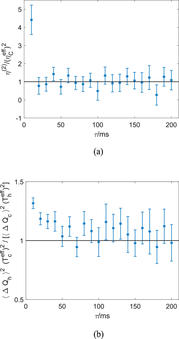
Comparison between the theoretical results and the experimental data for the cycle period ranging from 10 to 200 ms. a Ratio ({eta }^{(2)}/{({eta }_{{{rm{C}}}}^{{{rm{eff}}}})}^{2}) obtained from experimental data of the position of the Brownian particle, which is around unity for large τ as predicted by Eq. (1). b The ratio (langle {(Delta {Q}_{{{rm{h}}}}^{exp })}^{2}rangle {({T}_{{{rm{c}}}}^{{{rm{eff}}}})}^{2}/[leftlangle {(Delta {Q}_{{{rm{c}}}}^{exp })}^{2}rightrangle {({T}_{{{rm{h}}}}^{{{rm{eff}}}})}^{2}]) is around unity for large τ as predicted by Eq. (2). The error bars in both panels show the standard error (s.e.m.).
Discussion
Statistical characterization of the engine’s performance using higher-order moments beyond the mean values is a key issue for understanding the thermodynamics of the mesoscale. We have derived universal relations (1) and (4) between fluctuations (higher-order central moments) of work and heat in the Carnot cycle. We have also shown that the Carnot cycle provides the universal upper bound for the ratio between the variances of work and heat [Eq. (9) for an arbitrary quasistatic cycle and Eq. (11) for a large class of quasistatic cycles, including most of the typical cycles]. This bound might hold even for a wider class of heat engines than those considered in the present work, since the relation similar to Eq. (1) also holds for steady-state heat engines with nonzero power output58,59. Furthermore, our experimental test suggests that the results obtained in our work can still hold beyond the quasistatic regime. In addition, our results are applicable to study irreversible non-quasistatic cases through the endo-reversible formalism60,61.
Our results provide a guiding principle in the design of reliable and energy-efficient microscopic heat engines, which is an important problem for various topics relevant to the thermodynamics of small systems6,22,23,24. From the relations (1) and (11), we have ({leftlangle Delta {W}^{2}rightrangle }^{1/2}le {eta }_{{{rm{C}}}},{leftlangle Delta {Q}_{{{rm{h}}}}^{2}rightrangle }^{1/2}). This indicates that we can reduce the fluctuations of the total work output by reducing the fluctuations of heat (leftlangle Delta {Q}_{{{rm{h}}}}^{2}rightrangle) in the heat-exchanging stroke(s) with the hot heat bath. For a working substance with the number of states in the form of Iλ(E) = f(λ) Eα as an example, this can be achieved, e.g., by using a trap potential giving a smaller value of α: for example, using a box potential (α = 1/2) instead of a harmonic oscillator one (α = 1) in one dimension.
Let us illustrate this scheme by taking the Carnot cycle as an example. From Eq. (1), we have (leftlangle Delta {W}^{n}rightrangle ={eta }_{{{rm{C}}}}^{n}leftlangle Delta {Q}_{{{rm{h}}}}^{n}rightrangle). Since the mean value of the heat input, Qh through the quasistatic isothermal stroke depends only on the temperature Th and λ but is independent of α as (leftlangle {Q}_{{{rm{h}}}}rightrangle ={k}_{{{rm{B}}}}{T}_{{{rm{h}}}}ln [f({lambda }_{1})/f({lambda }_{0})]) (see the subsection “Average and fluctuation of heat input through a quasistatic isothermal stroke for a working substance with Iλ(E) = f(λ)Eα ” in the “Methods” section), so it is for the mean value of the total work output (leftlangle Wrightrangle ={eta }_{{{rm{C}}}}leftlangle {Q}_{{{rm{h}}}}rightrangle). On the other hand, the fluctuation of Qh depends only on Th and α as (leftlangle Delta {Q}_{{{rm{h}}}}^{2}rightrangle =2{({k}_{{{rm{B}}}}{T}_{{{rm{h}}}})}^{2}alpha) (see the “Methods” section). Therefore, by decreasing α, we can reduce the fluctuation (leftlangle Delta {W}^{2}rightrangle) without reducing the average total work output W and efficiency. In addition to the variance, higher moments (leftlangle Delta {W}^{n}rightrangle) with n > 2 which describe, e.g., the skewness (n = 3) and the kurtosis (n = 4) from the Gaussian distribution, can also be reduced at the same time in the above way since the higher moments of (leftlangle Delta {Q}_{{{rm{h}}}}^{n}rightrangle) with n > 2 also depends only on Th and α [e.g., (leftlangle Delta {Q}_{{{rm{h}}}}^{3}rightrangle =4{({k}_{{{rm{B}}}}{T}_{{{rm{h}}}})}^{3}alpha), (leftlangle Delta {Q}_{{{rm{h}}}}^{4}rightrangle =6{({k}_{{{rm{B}}}}{T}_{{{rm{h}}}})}^{4}alpha (alpha +2)), etc.]. Therefore, the above scheme is beneficial not only for the variance but also for all the moments of ΔW.
As the probability distribution function (pdf) of W for microscopic heat engines significantly deviates from the Gaussian (see, e.g., Fig. S1 of ref. 4; note that, while the pdf of the phase space variables is Gaussian, it is not the case for W), several higher order moments of (leftlangle Delta {W}^{n}rightrangle) for n = 3 and n = 4 are also important to characterize the performance of the heat engines. The relation (1) can potentially provide another guiding principle to deal with these higher moments. Finding a scheme to control these higher moments separately from the variance would be an interesting future issue.
Methods
Fluctuations of work and heat in the quasistatic isothermal process
It has been discussed that the fluctuation of work output throughout the quasistatic isothermal process vanishes as ~O(τ−1/2) for a long duration τ of the process16,53,62. Namely, in the limit of large τ, each sample path gives the same value of the work for a given protocol in the quasistatic isothermal process. This is because there is no long-time correlation in the variation of the force exerted by the working substance: this force varies due to thermal fluctuation caused by contact with a heat bath, and thus the variation does not have a long-time correlation. In the following, we shall show this vanishing fluctuation using the path integral representation.
Let us consider a trajectory γ in the phase space between the initial time tinit and the final time tfin under the driving of an external control parameter λ(t) (whose initial and the final values are λinit and λfin, respectively). The work output W from the system along this trajectory is given by
The first and the second moments of the work averaged over sample paths are
where ({{mathcal{P}}}[gamma ]) is the probability (density) of the trajectory γ, and (int,{{mathcal{D}}}Gamma) denotes the functional integral with respect to the trajectories.
We set the duration of the process as τ ≡ tfin−tinit = Mτunit with M being an integer and τunit being a sufficiently long time so that the variation of the parameter λ is slow enough. (As a prerequisite, τunit is taken to be much larger than the correlation time τcorr of the thermal fluctuation of the force.) Then we shall see the variance (leftlangle Delta {W}^{2}rightrangle) of work W vanishes for large M. To evaluate the right-hand side of Eqs. (13) and (14), we discretize the time τunit into a sufficiently large number of N + 1 points, {t0 ≡ tinit, t1, t2, ⋯ , tN ≡ tinit + τunit}, by the time step Δt ≡ tn+1−tn= τunit/N, which is taken to be much larger than the correlation time τcorr so that the force exerted by the working substance at different time slices tn is uncorrelated. Therefore, the probability density ({{mathcal{P}}}[gamma ]) of the trajectory can be written as a product of the phase space distribution function ({P}_{{lambda }_{n}}({Gamma }_{n};,{t}_{n})) at each time slice tn. The phase space point and the external parameter at time tn (0 ≤ n ≤ MN) are denoted by Γn ≡ (qn, pn) and λn, respectively. Here, q and p represent the D generalized coordinates and momenta, respectively, in the 2D-dimensional phase space for the system with D degrees of freedom. Then ({{mathcal{D}}}Gamma) reduces to ({{mathcal{D}}}Gamma to {prod }_{n = 0}^{MN}d{Gamma }_{n}), where dΓn ≡ Cdqn dpn is the phase space volume element at time tn including the numerical factor C coming from the phase space volume of a microstate.
Thus, the average of work (leftlangle Wrightrangle) given by Eq. (13) reads
where Δλi with 0 ≤ i ≤ N sets the protocol of the parameter change in the case of τ = τunit with M = 1: Δλi ≡ λi+1−λi if i = m/M is an integer; otherwise, Δλm/M is between Δλ[m/M] and Δλ[m/M]+1, where [m/M] is the integer part of m/M. Note that the factor of 1/M appears because the speed of the parameter change is slowed down by increasing the total duration τ of the process by a factor of M. Similarly, the second moment (14) becomes
Here, the second and the third terms of the right-hand side scales as ~1/M since the summation ({sum }_{m = 0}^{MN-1}) yields a contribution of a factor of M, which is multiplied by the factor of 1/M2.
From Eqs. (15) and (16), we readily see that the variance of work (leftlangle Delta {W}^{2}rightrangle) in the quasistatic isothermal process is given by the second and the third terms of Eq. (16) both of which scale as ~1/M and have an opposite sign with each other. Therefore, the variance (leftlangle Delta {W}^{2}rightrangle) vanishes as ~τ−1 or faster:
or the fluctuation ΔW vanishes as (sqrt{leftlangle Delta {W}^{2}rightrangle }=O({tau }^{-1/2})). As a consequence, fluctuation of W through the quasistatic isothermal process becomes negligible provided the duration τ of the process is sufficiently long, and (leftlangle Delta {W}^{2}rightrangle to 0) in the limit of τ → ∞.
Next, we shall also discuss the fluctuation of heat during the quasistatic isothermal process. From the first law of thermodynamics for an individual trajectory, the heat absorbed by the system along the trajectory γ is given by
where Γinit and Γfin are the initial and the final phase space points of the trajectory γ. The first and the second moments of the heat averaged over sample paths are
The average of heat (19) can be written as
where (leftlangle Wrightrangle) is given by Eq. (15), and ({leftlangle Arightrangle }_{lambda ,t}equiv int,dGamma ,,{P}_{lambda }(Gamma ;,t),A(Gamma ),) is the average of “A” at time t.
Similarly, the second moment (20) reads
Here, the fifth term on the right-hand side can be written as
Note that, for the variance (leftlangle Delta {Q}^{2}rightrangle equiv leftlangle {Q}^{2}rightrangle -{leftlangle Qrightrangle }^{2}) of heat Q, the contribution from the first term in the right-hand side of Eq. (23) cancels and only those from the second and the third terms remain, which scale as ~1/M. Therefore, from Eqs. (21)–(23), the variance of heat in the quasistatic isothermal process reads
with ({leftlangle Delta {H}_{lambda }^{2}rightrangle }_{lambda ,t}equiv {leftlangle {H}_{lambda }^{2}rightrangle }_{lambda ,t}-{({leftlangle {H}_{lambda }rightrangle }_{lambda ,t})}^{2}). Thus, (leftlangle Delta {Q}^{2}rightrangle to {langle Delta {H}_{{lambda }_{{{rm{fin}}}}}^{2}rangle }_{{lambda }_{{{rm{fin}}}},{t}_{{{rm{fin}}}}}+{langle Delta {H}_{{lambda }_{{{rm{init}}}}}^{2}rangle }_{{lambda }_{{{rm{init}}}},{t}_{{{rm{init}}}}}) in the limit of τ → ∞.
Derivation of Eqs. (1), (2), and (4)
In this subsection, we provide the detailed derivation of the universal relations, Eqs. (1), (2), and (4), of the central moments of work and heat for the reversible Carnot cycle. The four strokes of the reversible Carnot cycle (Fig. 4) are performed as follows. (0): Initial state: First, we set the external parameter at λ0 and start with a randomly chosen microstate from the canonical ensemble for ({H}_{{lambda }_{0}}) at temperature Th. (0+ → 1−): Quasistatic isothermal expansion: We make a thermal contact between the engine and the hot heat bath with temperature Th, then slowly increase the parameter from λ0 to λ1. (1+ → 2−): Quasistatic adiabatic expansion: We remove the thermal contact between the engine and the bath and slowly increase the parameter from λ1 to λ2. (2+ → 3−): Quasistatic isothermal compression: At point 2+, we make a thermal contact between the engine and the cold heat bath with temperature Tc, then decrease the parameter from λ2 to λ3. (3+ → 4−): Quasistatic adiabatic compression: We remove the thermal contact between the engine and the bath and decrease the parameter from λ3 to λ4. Here, point 4− is equivalent to point 0: the parameter returns to the initial value, i.e. λ4 = λ0, and the phase space distribution functions at points 4− and 0 are the same to close the cycle. Here, we do not include the contribution from point 4+ which becomes negligible for a continuous operation over consecutive cycles.
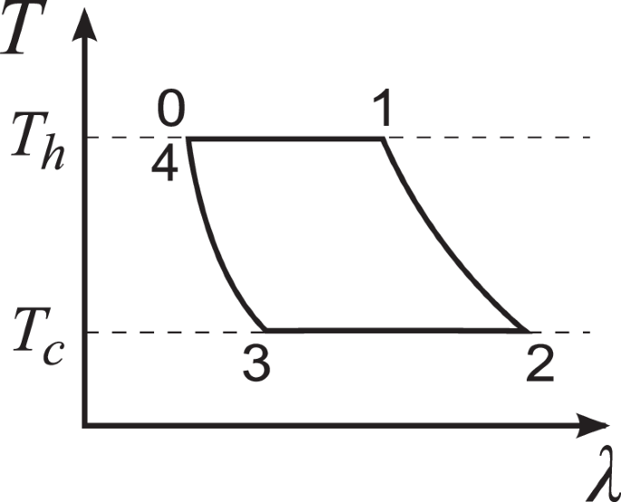
The temperature versus external control parameter (T−λ) diagram of the Carnot cycle working with a hot heat bath at temperature Th and a cold one at Tc.
In general, work and heat through each stroke, and the internal energy of the initial and the final states of each stroke are random variables. However, fluctuation ΔWisoth of the work output Wisoth through the quasistatic isothermal process becomes negligible if the duration τ of the process is sufficiently long16,53 (see also the subsection “Fluctuations of work and heat in the quasistatic isothermal process” in the “Methods” section), and it vanishes no slower than ~τ−1/2, i.e., (Delta {W}_{{{rm{isoth}}}}equiv {W}_{{{rm{isoth}}}}-leftlangle {W}_{{{rm{isoth}}}}rightrangle =O({tau }^{-1/2})). This is because there is no long-term correlation in the variation of the force exerted by the working substance16. Let us now focus on the quasistatic isothermal expansion stroke 0+ → 1−. From the first law of thermodynamics, work output W0→1 by the engine, heat input Qh from the hot heat bath to the working substance, and the internal energy of the working substance ({E}_{0}^{+}) and ({E}_{1}^{-}) at the initial and the final state of the stroke should satisfy
Since the fluctuation of W0→1 is negligible (i.e., ({W}_{0to 1}=leftlangle {W}_{0to 1}rightrangle)) while Qh, ({E}_{0}^{+}), and ({E}_{1}^{-}) are not the case, we obtain
Here, (leftlangle {Q}_{{{rm{h}}}}rightrangle) is the ensemble average of Qh over possible sample paths, and (leftlangle {E}_{i}^{pm }rightrangle) is the average of ({E}_{i}^{pm }) over the canonical ensemble at point i±. Note that ({E}_{i}^{+}={E}_{i}^{-}) because of the first law of thermodynamics together with the fact that the work for making and removing a thermal contact with a heat bath is negligible16. [However, (leftlangle {E}_{i}^{+}rightrangle =leftlangle {E}_{i}^{-}rightrangle) is sufficient to prove the universal relations (1), (2), and (4). The condition ({E}_{i}^{+}={E}_{i}^{-}) is required only in the proof of the universal bounds given by Eqs. (9) and (11).]
Next, we consider the total work output W through the whole cycle:
where Wi→i+1 is work output through the stroke from point i+ to (i + 1)−. Since the fluctuations of W0→1 and W2→3 by the quasistatic isothermal strokes are negligible, we obtain
Here, the strokes 1+ → 2− and 3+ → 4− are quasistatic adiabatic processes. Since there is no heat exchange between the working substance and the heat bath during these strokes, W1→2, for example, reads
In addition, for our working substance, since the initial and the final state of the quasistatic adiabatic stroke should satisfy the AR condition, we have ({E}_{1}^{+}/{T}_{{{rm{h}}}}={E}_{2}^{-}/{T}_{{{rm{c}}}}). From this relation and Eq. (29), we get
Similarly, for the stroke 3+ → 4−, we get ({W}_{3to 4}={E}_{3}^{+}-{E}_{4}^{-}=left[({T}_{{{rm{c}}}}/{T}_{{{rm{h}}}})-1right],{E}_{4}^{-}). Thus Eq. (28) reads
From Eqs. (26) and (31) together with the fact that ({E}_{0}^{+}) and ({E}_{4}^{-}) are statistically equivalent random variables (i.e., random variables following the same probability distribution function), we finally obtain Eq. (1):
for any integer n ≥ 2.
For the quasistatic isothermal compression stroke 2+ → 3−, heat output Qc from the working substance to the cold heat bath through this stroke is given by
Since the fluctuation of W2→3 is negligible, we get
The AR condition for the quasistatic adiabatic strokes 1+ → 2− and 3+ → 4− reads ({E}_{1}^{+}/{T}_{{{rm{h}}}}={E}_{2}^{-}/{T}_{{{rm{c}}}}) and ({E}_{3}^{+}/{T}_{{{rm{c}}}}={E}_{4}^{-}/{T}_{{{rm{h}}}}), respectively. Since ({E}_{2}^{pm }) and ({E}_{3}^{pm }) are independent and ({E}_{2,3}^{-}={E}_{2,3}^{+}), Eq. (33) with the above conditions leads to Eq. (2):
which can be rewritten in the form analogous to the “central” relation of thermodynamics54, (leftlangle {Q}_{{{rm{h}}}}rightrangle /{T}_{{{rm{h}}}}=leftlangle {Q}_{{{rm{c}}}}rightrangle /{T}_{{{rm{c}}}}), as
Note that, since the temperatures Tc and Th are arbitrary, this relation holds for two arbitrary quasistatic isotherms connected by two quasistatic adiabats. The sum ΔQ(2) of the heat fluctuations over the separated sequences of heat exchanging strokes is given by [same as Eq. (3)]
From this equation and Eq. (1), we obtain Eq. (4):
Derivation of Eqs. (7) and (8)
Here we show the detailed derivation of Eqs. (7) and (8). Since the temperatures ({T}_{{J}_{i}}) and ({T}_{{J}_{i}+1}) (({T}_{{K}_{j}}) and ({T}_{{K}_{j}+1})) are in the region of [Tc,Th] and ({T}_{{J}_{i}}ge {T}_{{J}_{i}+1}) (({T}_{{K}_{j}+1}ge {T}_{{K}_{j}})), we get (1ge {T}_{{J}_{i}+1}/{T}_{{J}_{i}}ge {T}_{{{rm{c}}}}/{T}_{{J}_{i}}ge {T}_{{{rm{c}}}}/{T}_{{{rm{h}}}}) ((1ge {T}_{{K}_{j}}/{T}_{{K}_{j}+1}ge {T}_{{{rm{c}}}}/{T}_{{{rm{h}}}})). Therefore,
and
Applying these relations to Eqs. (5) and (6):
we finally obtain Eqs. (7) and (8):
Average and fluctuation of heat input through a quasistatic isothermal stroke for a working substance with I
λ(E) = f(λ)E
α
In this subsection, we derive the average and the fluctuation of heat input Qisoth in the quasistatic isothermal processes for a working substance with the number of states Iλ(E) = f(λ)Eα. Here, f is a function of the external parameter λ, and α is a real constant, which is fixed for each setup of the system. Namely, the form of f and the value of α are determined by, e.g., the shape of the trapping potential. For example, (f(d)=sqrt{8m},d) and α = 1/2 for a particle (mass m) in a 1-dimensional box potential with width d, and f(ω−1) = 2πω−1 and α = 1 for a particle in a 1-dimensional harmonic oscillator potential with frequency ω.
For the working substance with Iλ(E) = f(λ)Eα, the density of state gλ(E) reads
Then, the canonical distribution ({P}_{beta ,,lambda }^{{{rm{eq}}}}) at the inverse temperature β ≡ 1/kBT and the external parameter λ is
with Zβ, λ being the partition function given by
where (Gamma (alpha )equiv int_{!0}^{infty }{d}x,{x}^{alpha -1}{{{rm{e}}}}^{-x}) is the gamma function.
For the canonical distribution given by Eq. (38), the average of the internal energy Ei and of its square ({E}_{i}^{2}) at point i with temperature Ti and parameter λi can be calculated as
Therefore, the variance (leftlangle Delta {E}_{i}^{2}rightrangle) of Ei reads
Suppose the initial and the final nodes of the quasistatic isothermal stroke are denoted by points 1 and 2, the parameter λ at points 1 and 2 are denoted by λ1 and λ2, respectively, and the temperature of the working substance is constant at T. For the working substance considered, the average of the internal energy Ei of the working substance in an equilibrium state at point i in general is given by Eq. (40): (leftlangle {E}_{i}rightrangle ={k}_{{{rm{B}}}}{T}_{i}alpha). Therefore, for quasistatic isothermal strokes, the change in the average of the internal energy through the stroke is zero:
Thus, from the first law of thermodynamics, the average of the heat input Qisoth is equal to the average of the work output Wisoth through the quasistatic isothermal stroke:
For quasistatic isothermal processes, the work output given by Eqs. (12) and (13) reads
where
is the canonical distribution with respect to the phase space point Γ. From Eqs. (44) and (45), we finally get
The same result can also be obtained from the change in the entropy,
between the initial and the final states of the stroke:
Next, we derive the variance (leftlangle Delta {Q}_{{{rm{isoth}}}}^{2}rightrangle) of heat input through the quasistatic isothermal stroke for the working substance considered. According to Table 1, (leftlangle Delta {Q}_{{{rm{isoth}}}}^{2}rightrangle) is given by a sum of the variances of the internal energy at the initial and the final states of the stroke. From Eq. (42) with T ≡ T1 = T2, we obtain
From Eqs. (47) and (50), we can see that the mean value (leftlangle {Q}_{{{rm{isoth}}}}rightrangle) of the heat input Qisoth through the quasistatic isothermal stroke depends only on T and λ while its variance (leftlangle Delta {Q}_{{{rm{isoth}}}}^{2}rightrangle) depends only on T and α.
Integral fluctuation theorems and ({eta }_{{{rm{C}}}}^{(n)})
Following the treatment in ref. 55, the Jarzynski equality can be extended to the system coupled with two heat baths. Assuming that the coupling Hamiltonians between the system and the baths are negligible (the so-called weak-coupling case), the resulting integral fluctuation theorem reads56 (see also refs. 63,64)
with the stochastic entropy production Σ, including the total entropy change in the system and the baths through the whole process whose specific form will be defined below. Note that Eq. (51) is applicable to the protocol where the cycle starts with a canonical state at some temperature and the system is equilibrated again at the same temperature as the initial one at the end of the whole process.
For reversible processes such as the Carnot cycle considered in the present work which satisfies the AR condition, it is known that the mean value of the entropy production is zero:
From Jensen’s inequality together with Eq. (52), the lhs of Eq. (51) leads to
Therefore, for reversible processes we obtain
with (leftlangle Sigma rightrangle =0). One can show that Eqs. (52) and (54) simultaneously hold if and only if the stochastic entropy production Σ is deterministically zero:
for any sample path, i.e., the distribution function PΣ(σ) of Σ is
where δ is the Dirac delta function.
For a cyclic protocol starting from the canonical state at Tc (protocol 1), Σ in Eq. (51) is given by
On the other hand, Σ for a protocol starting from the canonical state at Th (protocol 2) is
Here, the superscripts “[i]” (i = 1 and 2) in Eqs. (57) and (58) mean the random variables associated to protocol i. As has been pointed out below Eq. (4), it is noted that the random variables in Eqs. (57) and (58) for different initial points (e.g., W[1] and W[2]) should be regarded as different random variables, which belong to different ensembles. This is clear from the fact that the fluctuation ΔE of the internal energy change through one cycle, E = (Qh−Qc)−W, depends on the temperature of the initial point so that work and heat for different protocols with different initial points are different random variables, which could have a different amount of fluctuations. Unlike the mean values, which are constrained by (leftlangle Erightrangle =0) for a cycle, there is no such a constraint on the fluctuations. Therefore, in the discussion of the fluctuations for a single cycle, the effects of the end points of the process are important.
From Eq. (55) and (57), we obtain
and similarly from Eq. (55) and (58), we obtain
Thus, from Eq. (59), we can obtain the universal relation of η(n) given by Eq. (1) for protocol 1:
where ({leftlangle cdots rightrangle }_{i}) represents the ensemble average of protocol i. However, it is not trivial to derive the same relation for different protocols with an initial state other than the canonical state at Tc from the integral fluctuation theorem.
Regarding the other universal relations given by Eqs. (2) and (4), it is also non-trivial to derive these relations from the integral fluctuation theorem since W[1] and W[2] in Eqs. (59) and (60) are different random variables so that ({leftlangle {(Delta {W}^{[1]})}^{n}rightrangle }_{1}) and ({leftlangle {(Delta {W}^{[2]})}^{n}rightrangle }_{2}) cannot be identified trivially.
Unlike the above derivation based on the integral fluctuation theorem, all the random variables of W, Qh, and Qc for the same protocol can be handled at the same time in the bottom-up approach employed in the subsection “Derivation of Eqs. (1), (2), and (4)” of the “Methods” section. In addition, with this bottom-up approach, deriving the relations (1), (2), and (4) for any other initial point is straightforward.
Comparison with experimental data
Correspondence relations
We provide a detailed derivation of the correspondence relations between the work distribution of the true adiabatic process in the Carnot cycle and the heat distribution of the isentropic process in the Brownian Carnot cycle (hereafter, Brownian isentropic process for short)4 in the quasistatic limit. In both the true adiabatic process and the Brownian isentropic process, the Shannon entropy is constant, and the system is in a canonical state throughout the process in the quasistatic limit. Therefore, for these processes starting at the same temperature T and the external parameter λ, their paths on the T−λ plane are the same.
Regarding the true adiabatic process, since the working substance is isolated during the process, its work output ({W}_{{{rm{ad}}}}^{{{rm{true}}}}) is given by
where Einit (Efin) and Tinit (Tfin) are the energy and temperature of the initial (final) state of the true adiabatic process, respectively. Here, we have used the AR condition, Einit/Tinit = Efin/Tfin, for the second equality. Since the probability distribution of Einit is the canonical state with the inverse temperature ({beta }_{{{rm{init}}}}={({k}_{{{rm{B}}}}{T}_{{{rm{init}}}})}^{-1}), i.e. (P({E}_{{{rm{init}}}})propto {{{rm{e}}}}^{-{beta }_{{{rm{init}}}}{E}_{{{rm{init}}}}}) (Einit > 0), the work distribution function ({P}_{{W}_{{{rm{ad}}}}^{{{rm{true}}}}}(w)) reads
for w > 0 [w ≤ 0] and ({P}_{{W}_{{{rm{ad}}}}^{{{rm{true}}}}}(w)=0) for w ≤ 0 [w > 0] when Tinit > Tfin (quasistatic adiabatic expansion) [Tinit ≤ Tfin (quasistatic adiabatic compression)].
On the other hand, in the Brownian isentropic process, which is an experimental counterpart of the true adiabatic process35, the working substance is always in contact with a heat bath with continuously variable temperature. In this process, the temperature and the external parameter λ are controlled simultaneously to maintain the Shannon entropy of the working substance constant. As has been derived in the supplementary material of ref. 35, the probability distribution function of the heat input through the Brownian isentropic process in the underdamped case (as in our experiment4) is given by
Here, (leftlangle {W}_{{{rm{ise}}}}^{{{rm{Brow}}}}rightrangle) is the mean value of the work output through the Brownian isentropic process.
Now, we calculate the moments of work output in the true adiabatic process and heat input in the Brownian isentropic process. First, we consider the adiabatic expansion stroke 1+ → 2− (see Fig. 4) with Tinit = Th, Tfin = Tc, and Tinit > Tfin. The distribution function of work output ({W}_{1to 2}^{{{rm{true}}}}) through the true adiabatic process, ({P}_{{W}_{1to 2}^{{{rm{true}}}}}(w)), and that of the heat input ({Q}_{1to 2}^{{{rm{Brow}}}}) through the corresponding Brownian isentropic process, ({P}_{{Q}_{1to 2}^{{{rm{Brow}}}}}(q)), are as follows:
with ΔT ≡ Th−Tc. From these distribution functions, the mean values of ({W}_{1to 2}^{{{rm{true}}}}) and ({Q}_{1to 2}^{{{rm{Brow}}}}) are calculated as
and
Thus, the relation between the mean values of ({W}_{1to 2}^{{{rm{true}}}}) and ({Q}_{1to 2}^{{{rm{Brow}}}}) reads
Similarly, for the second moments of ({W}_{1to 2}^{{{rm{true}}}}) and ({Q}_{1to 2}^{{{rm{Brow}}}}), we obtain
and
From Eqs. (67), (68), (70), and (71), we obtain the relation between the variances of ({W}_{1to 2}^{{{rm{true}}}}) and ({Q}_{1to 2}^{{{rm{Brow}}}}):
In the same way, we obtain the relations for the 3rd and 4th moments:
and
For the adiabatic compression stroke 3+ → 4− (see Fig. 4), following the same procedure, we obtain the similar relations between ({W}_{3to 4}^{{{rm{true}}}}) and ({Q}_{3to 4}^{{{rm{Brow}}}}):
Evaluation of η
(2) from experimental data
Now, we discuss the evaluation of η(2) using experimental data of the Brownian Carnot engine4. For the Carnot cycle in the quasistatic limit, the variance of total work output W through one cycle comes solely from the true adiabatic strokes:
where i = 1 → 2 (i = 3 → 4) for the adiabatic compression (expansion). To evaluate (leftlangle Delta {W}^{2}rightrangle) from the experimental data, we use the relations (72) and (76) between the work variance (langle {(Delta {W}_{i}^{{{rm{true}}}})}^{2}rangle) of the true adiabatic strokes and the heat variance (langle {(Delta {Q}_{i}^{{{rm{Brow}}}})}^{2}rangle) of the corresponding Brownian isentropic strokes. In the analysis, we identify the sample variance ({langle Delta {Q}_{i}^{2}rangle }_{exp }) of the experimental data of heat in the Brownian isentropic strokes with (langle {(Delta {Q}_{i}^{{{rm{Brow}}}})}^{2}rangle). In addition, since the actual effective temperature of the working substance in the isothermal strokes generally deviates from the temperature of the bath in the non-quasistatic regime, we use the time average of the effective temperature of the working substance during the hot (cold) isothermal stroke in the experiment, denoted by ({T}_{{{rm{h}}}}^{{{rm{eff}}}}) (({T}_{{{rm{c}}}}^{{{rm{eff}}}})), for Th(Tc) in these relations. (Note that ({T}_{{{rm{h}}}}^{{{rm{eff}}}}) and ({T}_{{{rm{c}}}}^{{{rm{eff}}}}) converge to the temperatures of the baths in the quasistatic limit.) As a consequence, we employ the following relation:
Hereafter, for the sample variance of some quantity O over the experimental realizations, we write ({leftlangle Delta {O}^{2}rightrangle }_{exp }) for clarity.
The variance ({langle Delta {Q}_{i}^{2}rangle }_{exp }) of heat can be decomposed into the variance ({langle Delta {Q}_{{{rm{k}}},i}^{2}rangle }_{exp }) of the kinetic energy and the variance ({langle Delta {Q}_{{{rm{p}}},i}^{2}rangle }_{exp }) of the potential energy: ({langle Delta {Q}_{i}^{2}rangle }_{exp }={langle Delta {Q}_{{{rm{k}}},i}^{2}rangle }_{exp }+{langle Delta {Q}_{{{rm{p}}},i}^{2}rangle }_{exp }). Here, dQp,i = −∂xV(x,λ)dx is obtained from the trajectory x(t) realized in the experiment. Since the relaxation time of the velocity of the Brownian particle is much shorter than the other time scales, we can assume that the kinetic energy is always distributed as in equilibrium with the environment. Thus, we obtain ({langle Delta {Q}_{{{rm{k}}},i}^{2}rangle }_{exp }={langle Delta {E}_{{{rm{k}}},{{rm{init}}}}^{2}rangle }_{exp }+{langle Delta {E}_{{{rm{k}}},{{rm{fin}}}}^{2}rangle }_{exp }=frac{1}{2}{k}_{{{rm{B}}}}^{2}({T}_{{{rm{init}}}}^{2}+{T}_{{{rm{fin}}}}^{2})) from the variance of the kinetic energy, Ek,init and Ek,fin, at two ends of each Brownian isentropic stroke, where Tinit =Th and Tfin = Tc for i = 1 → 2 (Tinit = Tc and Tfin = Th for i = 3 → 4). Consequently, ({langle Delta {Q}_{i}^{2}rangle }_{exp }) for the Brownian isentropic stroke is given by
Similarly, the variance of heat during the hot isothermal stroke (2 → 3), where Tinit = Tfin = Th, is given by
From Eqs. (79), (80), (81), and (82), we finally obtain η(2) as
which we evaluate by using the experimental data of ({langle Delta {Q}_{{{rm{p}}},i}^{2}rangle }_{exp }), ({T}_{{{rm{h}}}}^{{{rm{eff}}}}), and ({T}_{{{rm{c}}}}^{{{rm{eff}}}}).
Evaluation of sampling error
Due to the finite number of samples (i.e., a finite number of realizations of trajectories), the sample variance ({langle Delta {Q}_{{{rm{p}}}}^{2}rangle }_{exp }) of Qp obtained from the sample trajectories can deviate from the theoretical value of the variance (langle {(Delta {Q}_{{{rm{p}}}}^{{{rm{Brow}}}})}^{2}rangle). To calculate the error bars shown in Fig. 3, we simulate this deviation due to the finite number of trajectories realized in the experiment as follows.
In the quasistatic limit, we assume Qp = Ep,fin−Ep,init, where the probability density function of the potential energy Ep,j at node j is given by (P({E}_{{rm p}, j})={(pi {k}_{{{rm{B}}}}{T}_{j} {E}_{{rm p}, j})}^{-1/2}exp (-{E}_{{rm p}, j}/{k}_{{{rm{B}}}}{T}_{j})). We evaluate the error in ({langle Delta {Q}_{{{rm{p}}}}^{2}rangle }_{exp }) caused by the finite number of samples in the experiment by a Monte–Carlo simulation based on this P(Ep,j). From the errors of ({langle Delta {Q}_{{{rm{p}}},1to 2}^{2}rangle }_{exp }), ({langle Delta {Q}_{{{rm{p}}},2to 3}^{2}rangle }_{exp }), and ({langle Delta {Q}_{{{rm{p}}},3to 4}^{2}rangle }_{exp }) obtained by the simulation, the error of η(2) is finally obtained through the error propagation formula for Eq. (83).
Responses