Universal validity of the second law of information thermodynamics

Introduction
The problem of consistency between the second law of thermodynamics and information processing has been at the center of one of the longest running debates in the history of modern physics, ever since Maxwell conjured up his famous demon1. A widely accepted solution to Maxwell’s paradox is that consistency with the second law of thermodynamics is recovered by taking into account the work cost for measurement and erasure, i.e., the resetting of the demon’s memory to its initial state2,3,4,5,6,7,8. These ideas, bridging thermodynamics with information theory, are nowadays collectively referred to as information thermodynamics9,10.
In this context, and including a quantum theoretical scenario, Sagawa and Ueda, in a series of celebrated papers11,12,13, derived an achievable upper bound for the work extracted by feedback control and showed that the conventional second law can, in general, be violated from the viewpoint of the system alone, but such a violation is exactly compensated by the cost of implementing the controlling measurement and resetting the memory. Such a tradeoff relation is what they call the second law of information thermodynamics (ITh).
Unfortunately, despite their importance, the balance equations established in refs. 11,12,13 rely on several mutually inconsistent assumptions that lack a direct operational interpretation. Moreover, these works only discuss sufficient conditions for the validity of such balance equations. While some generalizations and refinements have been proposed14,15,16,17,18,19,20,21,22, the demon’s memory readout process is always limited to ideal projective measurements. Besides being unrealistic in practice, such an assumption is problematic in principle: since the demon’s memory enters directly into the thermodynamic balance, the process acting on it must be treated in full generality, lest we obtain statements of limited scope. As a result, a comprehensive characterization of the validity range of the second law of ITh remains elusive, and it is unclear under what conditions the second law of ITh holds. In fact, at the time of writing, it is not even clear whether the second law of ITh should be considered a universal law or not, and what its logical status is with respect to the conventional second law of thermodynamics.
Our paper addresses this gap by adopting a top-down approach. Instead of attempting to derive the second law from assumptions with unclear logical necessity, we initiate from a purely information-theoretic framework and obtain balance equations that hold for any measurement and isothermal feedback process, in particular including any readout mechanism, and subsequently impose the second law of phenomenological thermodynamics as a constraint. This approach, which follows that used by von Neumann to derive his entropy’s equation23,24, allows us to determine exactly (in terms of sufficient and necessary conditions) how far feedback control and erasure protocols can be generalized while remaining overall consistent with the second law. We are then able to demonstrate the universal validity of the second law of ITh in general feedback control and erasure protocols: as long as such a protocol is compatible with the second law of phenomenological thermodynamics, it must also satisfy the second law of ITh, regardless of the measurement and feedback process involved.
A quantity that plays a crucial role in our analysis is the Groenewold–Ozawa information gain25,26: while previous works14,15,16,19,27,28 have also provided it with a thermodynamic interpretation—even in situations when it takes negative values—our balance equations show that such interpretation holds in complete generality.
Results
The minimum scenario required to discuss Maxwell’s paradox and feedback control protocols in full generality, but without oversimplifications, comprises five systems, as shown in Fig. 1: the physical system (i.e., the gas) being measured, denoted by A; the controller’s (i.e., the demon’s) internal state M (where the letter “M” stands for “Maxwell”, “measurement apparatus” or “memory”); a classical register K recording the measurement’s outcomes; and two independent baths B1 and B2 (one used during the feedback control stage, the other used for the final erasure of the measurement), which are assumed to be at the same finite temperature. This means that the overall process is assumed to be isothermal.

the target system A, the controller (demon) consisting of an internal state M and a classical register K, and two baths B1 and B2 at the same inverse temperature β.
Without any feedback control, for isothermal processes, the second law of thermodynamics is equivalent to the statement that the work extracted from the system A can reach but not exceed the change in the free energy(These and other key concepts will be rigorously introduced and discussed in what follows. The purpose of these first few paragraphs is simply to provide a relatively informal overview of our main findings). of the system—in formula, ({W}_{{rm{ext}}}^{A}leqslant -Delta {F}^{A}). The main contribution of ref. 11 was to show that if feedback control is allowed instead, the work extracted can go all the way up to ({W}_{{rm{ext}}}^{A}=-Delta {F}^{A}+{beta }^{-1}{I}_{{mathrm{QC}}}), where IQC is a non-negative term quantifying the amount of information collected by the measurement used to guide the subsequent feedback control protocol. In this sense, Maxwell’s demon can indeed violate the second law of thermodynamics, but this conclusion should come as no surprise, since the demon is not yet included in the global thermodynamic balance at this point.
Indeed, once the demon itself is embodied in a physical system, such a violation of the second law turns out to be only a local violation, which is perfectly possible as long as it is compensated for elsewhere. According to Landauer’s principle, such a compensation should be identified with the cost of performing the measurement and resetting the measurement apparatus and register at the end of the protocol, so that they are ready for use in the next round. Following this narrative, refs. 12,13 list a number of assumptions about the quantum feedback protocol so that, as one would expect, the work cost of implementing the measurement and performing its erasure is lower bounded as ({W}_{{rm{in}}}^{MK}geqslant {beta }^{-1}{I}_{{mathrm{QC}}}), thus guaranteeing that the total net work extracted ({W}_{{mathrm{tot}}}:={W}_{{rm{ext}}}^{A}-{W}_{{rm{in}}}^{MK}leqslant -Delta {F}^{A}) is still within the limits of the second law of thermodynamics.
Our analysis begins by removing all assumptions from the consistency argument above. We argue that this is not just for the sake of mathematical generality, but is necessary for two reasons. The first reason is that, specifically in relation to refs. 11,12,13, some of the assumptions made therein are, as we will show in what follows, extremely restrictive—so stringent, in fact, that they are inconsistent in most cases, constraining the analysis to trivial situations. The second reason is a matter of principle: if certain assumptions are required to restore the validity of the second law, the consistency between thermodynamics and quantum information processing cannot be considered universal, contrary to what folklore claims.
We then show that, when all assumptions about the mathematical form of the quantum feedback protocol are removed, the work extracted from the target system is upper bounded as
while the work cost of implementing the measurement and its erasure is now lower bounded as
where ΔSAMK denotes the entropy change of the entire compound AMK due to the measurement process and IGO is the Groenewold–Ozawa information gain25,26. Note that while the bound (1) looks similar to the one given in11, the information quantity IGO appearing in our bounds is different from the one used in refs. 11,12,13: in general, IGO ⋚ IQC. But while IQC does not provide the correct bounds in general, IGO does and, moreover, gives the same numerical values as IQC in all cases considered in11,12,13. Further, Eqs. (1) and (2) together imply that the net work extracted in general is bounded as
In other words, even if the final erasure is implemented in accordance with Landauer’s principle, the second law may still be violated whenever ΔSAMK < 0. Eqs. (1) and (2) constitute the main technical contributions of this work: their formal statement is given as Theorem 1 below.
Finally, by means of explicit counterexamples, we show that the axioms of quantum theory by themselves are perfectly consistent with a measurement process that decreases the total entropy of the system-memory-register compound, implying a violation of the second law according to Eq. (3). This leads us to the main conceptual contribution of this work, i.e. the conclusion that—contrary to some cursory accounts—in a quantum mechanical feedback process it is not enough to eventually perform an erasure process, as stipulated by Landauer’s principle, to guarantee the validity of the second law. In other words, the second law of thermodynamics is logically independent of the axioms of quantum theory, and its role is to constrain the set of possible measurement processes from the outset. Any attempt to prove the second law from within quantum theory is doomed to result in pure tautology29,30.
Framework
Consider a quantum system Y associated with a finite-dimensional Hilbert space ({{mathcal{H}}}^{Y}). The algebra of linear operators LY on ({{mathcal{H}}}^{Y}) will be denoted as ({mathcal{L}}({{mathcal{H}}}^{Y})), ({{mathbb{1}}}^{Y}) and ({{mathbb{O}}}^{Y}) denoting the unit and null operators, respectively. States on Y are represented by unit-trace positive operators, i.e., ({rho }^{Y}geqslant {{mathbb{O}}}^{Y}), Tr[ρY] = 1. A thermodynamic systemY is defined as the tuple (ρY; HY; β), where HY is the Hamiltonian and β: = 1/kBT > 0 is the inverse temperature of an external thermal bath, with kB Boltzmann’s constant. Throughout, we shall only consider the case where the thermal bath has a constant temperature, and so for notational simplicity we will abbreviate the thermodynamic system as (ρY; HY). When the system is in thermal equilibrium, the thermal state or Gibbs state is defined as ({gamma }^{Y}:={e}^{-beta {H}^{Y}}/{Z}^{Y}), where ({Z}^{Y}:={mathrm{Tr}}[{e}^{-beta {H}^{Y}}]) is the partition function.
The generalized quantum feedback control and erasure protocols we shall consider will comprise of five discrete time steps ti, i = 0, 1, 2, 3, 4. The total system is composed of a target system A, a controller consisting of a memory M and a classical register K, and two thermal baths B1, B2, both of which have the same inverse temperature β > 0, as depicted in Figure 1. For notational simplicity, we shall omit superscripts when denoting any quantity pertaining to the entire compound B1AMKB2, reserving their use only when discussing subsystems; for example, the state of subsystem AMK at time step ti will be denoted as ({rho }_{i}^{AMK}:={{mathrm{Tr}}}_{{B}_{1}{B}_{2}}[{rho }_{i}]), etc. In particular, we shall assume that the Hamiltonian at time step ti reads ({H}_{i}={H}^{{B}_{1}}+{H}_{i}^{A}+{H}^{MK}+{H}^{{B}_{2}}). That is, at each time step we assume that there are no interaction terms between the different subsystems, and only the Hamiltonian of the target system A may change. The protocol is represented schematically in Figure 2; below we shall describe each step in detail.
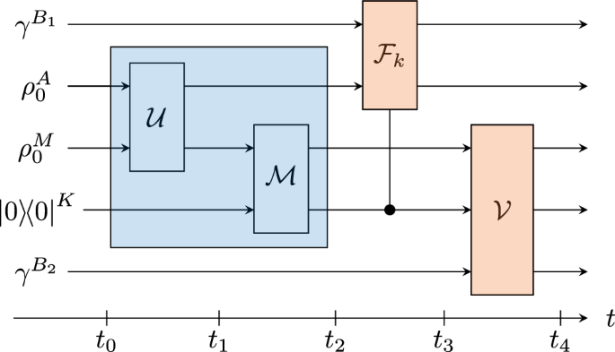
Interaction step (t0 → t1): system A and memory M interact by a unitary channel ({mathcal{U}}). Readout step (t1 → t2): an instrument ({mathcal{M}}) is applied on the memory M and the outcome k is written on the classical register K. The interaction step and the readout step together are referred to as the measurement step. Feedback control step (t2 → t3): a controlled unitary channel ({{mathcal{F}}}_{k}) is applied on the compound of system A and thermal bath B1 depending on the outcome k. Erasure step (t3 → t4): a unitary channel ({mathcal{V}}) is applied on the compound of MK and thermal bath B2, so as to return the state of MK to its initial configuration. The total compound system is assumed to evolve adiabatically during the entire protocol, that is, no heat is exchanged with any outside source.
The preparation step
At the initial time t = t0, the compound system is prepared in the state
where ({rho }_{0}^{A}) and ({rho }_{0}^{M}) are arbitrary states on A and M, respectively, while ({leftvert 0rightrangle }^{K}) represents the idle state of the classical register(Note that the memory considered in ref. 12 is described by a Hilbert space with a direct sum structure. Here we describe the degrees of freedom of the labels of the blocks and the internal states of the memory using different quantum systems. In the context of our paper, the two pictures are clearly equivalent.), and ({gamma }^{{B}_{1}},{gamma }^{{B}_{2}}) are the thermal states of the baths, with respect to the same inverse temperature β. Note that a common assumption is that the initial state of the memory ({rho }_{0}^{M}) is thermal at the same inverse temperature β as the two baths: while such an assumption is very reasonable from a physical point of view, and in particular facilitates the discussion of the erasure step (see below), for the sake of generality we keep ({rho }_{0}^{M}) arbitrary.
The measurement step
This step comprises an interaction step and a readout step. The interaction or pre-measurement step (from t = t0 to t = t1) represents the interaction between A and M, described by a unitary channel ({mathcal{U}}(cdot ):=U(cdot ){U}^{dagger }) acting in AM. The readout or pointer objectification step (from t = t1 to t = t2) is represented as a CP-instrument31 acting in M, namely, a family ({mathcal{M}}:={{{mathcal{M}}}_{k}:kin {mathcal{K}}}) of completely positive linear maps ({{mathcal{M}}}_{k}:{mathcal{L}}({{mathcal{H}}}^{M})to {mathcal{L}}({{mathcal{H}}}^{M})), labeled by the measurement outcomes (kin {mathcal{K}}), such that their sum ({{mathcal{M}}}_{{mathcal{K}}}:={sum }_{kin {mathcal{K}}}{{mathcal{M}}}_{k}) is trace-preserving, i.e., a channel. The instrument ({mathcal{M}}) is associated with a unique positive operator-valued measure (POVM) ({mathsf{M}}:={{{mathsf{M}}}_{k}:kin {mathcal{K}}}), with elements defined using the “Heisenberg picture” dual of ({{mathcal{M}}}_{k}) as ({{mathsf{M}}}_{k}:={{mathcal{M}}}_{k}^{* }({{mathbb{1}}}^{M})). Since the POVM ({mathsf{M}}) acts in the memory, it is referred to as the pointer observable. After M is measured by the instrument ({mathcal{M}}), the observed outcome k is recorded in the classical register. Such classical readouts are assumed to be all perfectly distinguishable, and thus are represented, following a common convention in quantum information theory32, by orthogonal pure states ({leftvert krightrangle }^{K}).
Accordingly, at t = t2 the state of the compound system reads
where idA denotes the identity channel acting in A, and
with
whenever the probability of obtaining outcome k satisfies
otherwise ({rho }_{2,k}^{AM}) can be defined arbitrarily.
We note that a fixed tuple (({{mathcal{H}}}^{M},{rho }_{0}^{M},{mathcal{U}},{mathcal{M}})) defines a measurement process or measurement scheme for an instrument ({mathcal{A}}:={{{mathcal{A}}}_{k}:kin {mathcal{K}}}) acting in the target system A, with the operations reading
In particular, we stress that an instrument on the target system ({mathcal{A}}:={{{mathcal{A}}}_{k}:kin {mathcal{K}}}) can be realized by means of infinitely many different measurement processes. One of the results of this work will be to show that the laws of thermodynamics constrain the latter, not the former.
Remark
The formalism of CP-instruments provides the most general readout (i.e., pointer objectification) procedure allowed by quantum theory. While general instruments in the target system A have been considered before, all previous works have focused on a restricted class of instruments acting in the memory M, namely, Lüders instruments compatible with a projection-valued measure (PVM), also known as “ideal projective measurements”12,13,14,15,16,17,18,19,20,21,22. ({mathsf{M}}) is a PVM if the effects ({{mathsf{M}}}_{k}) are mutually orthogonal projections, and the operations of the corresponding ({mathsf{M}})-compatible Lüders instrument read ({{mathcal{M}}}_{k}^{L}(cdot ):={{mathsf{M}}}_{k}(cdot ){{mathsf{M}}}_{k}). As shown by Ozawa31, every instrument acting in A admits a canonical measurement scheme, where ({rho }_{0}^{M}) is chosen to be pure and the pointer observable is chosen to be a PVM. But we stress that the pointer observable in a given measurement process need not be a PVM; and, even if it is, the instrument measuring it need not be of the Lüders form. In fact, it is well known that every observable ({mathsf{M}}) admits infinitely many ({mathsf{M}})-compatible instruments.
The feedback control step
From t = t2 to t = t3, a feedback control protocol is performed. This is implemented by coupling the compound AK with the thermal bath B1 by a unitary channel ({mathcal{F}}(cdot ):=F(cdot ){F}^{dagger }), defined by the unitary operator (Note that unitarity of F implicitly assumes that K is represented by a Hilbert space ({{mathcal{H}}}^{K}) of dimension equal to the number of measurement outcomes, i.e, (dim ({{mathcal{H}}}^{K})=| {mathcal{K}}|).).
Here, Fk are unitary operators on B1A, which induce the unitary channel ({{mathcal{F}}}_{k}(cdot ):={F}_{k}(cdot ){F}_{k}^{dagger }) conditional on the classical register having recorded outcome k. At time step t = t3, the state of the compound reads
where
Here, ({rho }_{3,k}^{{B}_{1}AM}=({{mathcal{F}}}_{k}^{{B}_{1}A}otimes {{rm{id}}}^{M})({gamma }^{{B}_{1}}otimes {rho }_{2,k}^{AM})). We shall say that the feedback process is pure unitary if we choose ({F}_{k}={{mathbb{1}}}^{{B}_{1}}otimes {F}_{k}^{A}), so that for each outcome the target system undergoes an isolated unitary evolution. In other words, a pure unitary feedback process does not involve the thermal bath. This is the case considered in, e.g., refs. 11,12,13. However, since Szilard2 onward, the traditional formulation typically considers a feedback protocol that is done in contact with a thermal bath, as we do here.
The erasure step
Lastly, the erasure process from t = t3 to t = t4 is modeled by coupling MK with the thermal bath B2 by a unitary channel ({mathcal{V}}(cdot ):=V(cdot ){V}^{dagger }). We naturally assume that ({H}_{3}^{A}={H}_{4}^{A}), since the target system A remains dormant. At time step t4, the state of the compound system will read
such that, by definition of “erasure”, ({rho }_{4}^{MK}={rho }_{0}^{MK}={rho }_{0}^{M}otimes leftvert 0rightrangle {leftlangle 0rightvert }^{K}). That is, the interaction between MK and the bath B2 returns the local state of MK back to its initial configuration. Such a setting appears in the context of Landauer’s principle4,33,34. If, in addition, it holds that ({rho }_{4}^{AMK}={rho }_{4}^{A}otimes {rho }_{0}^{M}otimes leftvert 0rightrangle {leftlangle 0rightvert }^{K}), i.e., if the correlations between A and MK are also erased, then we say that the erasure is perfect. Otherwise, we call the erasure partial. While in principle perfect erasure can always be achieved if a suitable bath is provided, it is a non-trivial problem to determine whether such a unitary erasure process always exists for a given bath. To alleviate this problem, we also consider here protocols that include partial erasure. As mentioned above when discussing the preparation step, a conceptually simpler situation occurs when the initial state of the memory is thermal at the same bath temperature, so that the erasure process can be intuitively understood as a thermalization process.
About injected and extracted work, and the assumption of overall adiabaticity
The internal energy of a thermodynamic system is E(ρY; HY): =Tr[ρYHY], and the non-equilibrium free energy35,36 is F(ρY; HY): = E(ρY; HY) − β−1S(Y)ρ, where (S{(Y)}_{rho }:=-{mathrm{Tr}}[{rho }^{Y}ln {rho }^{Y}]) is the von Neumann entropy23. When a thermodynamic system transforms from t = ti to t = tj as (({rho }_{i}^{Y};{H}_{i}^{Y})mapsto ({rho }_{j}^{Y};{H}_{j}^{Y})), we denote the increase in internal energy E, nonequilibrium free energy F, and entropy S as follows:
Definition 1
Consider a thermodynamic system which transforms as (({rho }_{i}^{Y};{H}_{i}^{Y})mapsto ({rho }_{j}^{Y};{H}_{j}^{Y})). The transformation is defined as adiabatic if it does not involve an exchange of heat with an external bath. In such a case, by the first law of thermodynamics, the work injected into (resp., extracted from) the system is defined as the increase (resp., decrease) in internal energy, i.e.,
In our formalism, all thermal baths (i.e., the systems B1 and B2) are treated as internal and so there are no external baths with which heat is exchanged. Moreover, following a well-established convention dating back to Szilard2 and von Neumann23, and routinely adopted until these days11,12,16,37,38,39, we assume that the pointer objectification implemented by the instrument ({mathcal{M}}) is also adiabatic, although it is obviously non-unitary. This may be justified if, for example, the objectification process is sufficiently fast with respect to the time scale required for heat to dissipate40. Concerning the rest, i.e., during the premeasurement, feedback, and erasure steps of the protocol, the total compound transforms by a global unitary channel which, by definition, does not involve an interaction with any external system, and so clearly no heat is exchanged here either. In conclusion, while the subsystem AMK exchanges heat with B1 and B2 during the feedback and erasure steps, respectively, we treat the total compound B1AMKB2 as transforming adiabatically during the entire protocol.
Since the total process is adiabatic, the net extracted work is identified with the decrease in internal energy of the entire compound, that is, Wtot = − ΔE0→4. Now we wish to split the contribution to the total work as that originating from the target system A and that originating from the controller MK. To this end, we note that the target system is involved only during the measurement and feedback steps, the controller is involved only during the measurement and erasure steps, the thermal bath B1 is involved only during the feedback step, and the thermal bath B2 is involved only during the erasure step. As such, we may write (see Methods, Section IV A)
where
is the work extracted from the target system, and
is the work injected into the controller.
General work bounds
Before providing general bounds for the work defined in Eqs. (11) and (12), let us first introduce some useful information-theoretic quantities. For any state ρA and a positive operator σA such that msupp(ρA) ⊆ msupp(σA), the Umegaki quantum relative entropy is defined by (D({rho }^{A}parallel {sigma }^{A}):={mathrm{Tr}}[{rho }^{A}(ln {rho }^{A}-ln {sigma }^{A})];geqslant; 0)41, which is non-negative due to Klein’s inequality42,43, and vanishes if and only if ρA = σA. The quantum mutual information of a bipartite state ρAB is defined as I(A : B)ρ: = S(A)ρ + S(B)ρ − S(AB)ρ ≡ D(ρAB∥ρA ⊗ ρB) ⩾ 0, with equality if and only if ρAB = ρA ⊗ ρB. On the other hand, the conditional quantum entropy of a bipartite state ρAB is defined as S(A∣B)ρ: = S(AB)ρ − S(B)ρ, which can be negative. The conditional quantum mutual information of a tripartite state ρABC is defined as I(A : C∣B)ρ: = S(A∣B)ρ + S(C∣B)ρ − S(AC∣B)ρ ⩾ 0, where the non-negativity follows from the strong subadditivity of the von Neumann entropy (see, e.g., ref. 32). Finally, we introduce the following information measure related to the measurement process on the target system:
Definition 2
The Groenewold–Ozawa information gain25,26 of the target system’s measurement process is defined as:
where the entropy of the post-measurement state of the target system conditioned by the classical register, (S{(A| K)}_{{rho }_{2}}), can equivalently be written as ({sum }_{k}{p}_{k}S({rho }_{2,k}^{A})), i.e., the average entropy of the posterior states of A.
Remark
Note that IGO is determined entirely by the prior system state ({rho }_{0}^{A}) and the instrument ({mathcal{A}}) acting in A as defined in Eq. (6). The Groenewold–Ozawa information gain is guaranteed to be non-negative for all prior states ({rho }_{0}^{A}) if and only if the instrument ({mathcal{A}}) is quasi-complete; ({mathcal{A}}) is called quasi-complete if for all pure prior states ({rho }_{0}^{A}), the posterior states ({rho }_{2,k}^{A}:={{mathcal{A}}}_{k}({rho }_{0}^{A})/{p}_{k}) are also pure. An example of a quasi-complete instrument is an efficient instrument, whereby each operation can be written with a single Kraus operator, i.e., ({{mathcal{A}}}_{k}(cdot )={L}_{k}(cdot ){L}_{k}^{dagger }). In general, therefore, IGO can be negative26.
The following proposition gives universally valid expressions for the work associated with feedback control and erasure protocols with a general quantum measurement process, independent of thermodynamics and from a purely information-theoretic point of view.
Proposition 1
In the generalized quantum feedback control and erasure protocol (Fig. 2), the extracted work from the system is
and the work needed to run the controller is
where
denote the irreversible entropy production associated with the isothermal feedback and erasure steps.
See Methods, Section IV B, for the proof. We immediately see that Eq. (14) contains, besides the usual free energy change, a correction term that arises from the specific implementation of measurement and feedback protocol. Similarly, Eq. (15) contains additional correction terms to the usual entropy change of target system and controller.
We note that an equality similar to Eq. (14) was obtained in ref. 14, except that there the entropy production ({S}_{{rm{irr}}}^{{B}_{1}}) as well as the mutual information (I{(A:K)}_{{rho }_{3}}) was missing. The term (I{(A:K)}_{{rho }_{3}}=S({rho }_{3}^{A})-{sum }_{kin {mathcal{K}}}{p}_{k}S({rho }_{3,k}^{A})) corresponds to the Holevo information of the conditional states of A after feedback44, which is non-negative and vanishes if and only if ({rho }_{3,k}^{A}={rho }_{3}^{A}) for all k. Reference 45 also derives a similar equality, but it uses the QC-mutual information, and not the Groenewold–Ozawa information gain.
From Proposition 1, by discarding terms that are always either positive or negative,we obtain universally valid bounds for injected and extracted work in quantum feedback control and erasure protocols, as well as necessary and sufficient conditions for their saturation.
Theorem 1
In the generalized quantum feedback control and erasure protocol (Fig. 2), the work extracted from the target system is upper bounded as
where the equality holds if and only if (I{(A:K)}_{{rho }_{3}}={S}_{{rm{irr}}}^{{B}_{1}}=0).The work cost to run the controller is lower bounded as
where the equality holds if and only if (I{(A:M| K)}_{{rho }_{2}}={S}_{{rm{irr}}}^{{B}_{2}}=0).
Remark
Let us discuss, by means of examples, the conditions under which the bounds in the above theorem can be saturated. A necessary condition for the equality in Eq. (16) is for the entropy production during the feedback step, ({S}_{{rm{irr}}}^{{B}_{1}}), to vanish. This will trivially be achieved if the feedback process is chosen to be pure unitary, i.e., so that for each outcome the target system undergoes an isolated unitary evolution, as assumed in11. However, note that in general this alone will not guarantee the other necessary condition for the equality in Eq. (16), i.e., a vanishing Holevo information (I{(A:K)}_{{rho }_{3}}). Recall that this quantity vanishes if and only if ({rho }_{3,k}^{A}={rho }_{3}^{A}) for all k, which implies that ({rho }_{3,k}^{A}={rho }_{3,k^{prime} }^{A}) for all (k,k^{prime}). But if the feedback process is pure unitary, then ({rho }_{3,k}^{A}={F}_{k}^{A}({rho }_{2,k}^{A}){F}_{k}^{Adagger }). Since unitary channels leave the von Neumann entropy invariant, and two states are identical only if their entropies are identical, it clearly follows that a necessary condition for a vanishing Holevo information given a pure unitary feedback process is for all the posterior states after measurement, ({rho }_{2,k}^{A}), to have the same entropy. While this can be achieved if, for example, the system undergoes a von Neumann measurement of a non-degenerate observable, for general measurement processes this is not the case. This is why in physically relevant situations, in order to saturate Eq. (16) a feedback process that exchanges entropy with a thermal bath is required, thus going beyond the paradigm of pure unitary feedback processes employed in11.
Remark
Similarly as above, a necessary condition for the equality in Eq. (17) is for the entropy production during erasure, ({S}_{{rm{irr}}}^{{B}_{2}}), to vanish. The other necessary condition, however, is given by a vanishing conditional mutual information (I{(A:M| K)}_{{rho }_{2}}={sum }_{kin {mathcal{K}}}{p}_{k},I{(A:M)}_{{rho }_{2,k}}). Clearly, such a quantity vanishes if and only if ({rho }_{2,k}^{AM}={rho }_{2,k}^{A}otimes {rho }_{2,k}^{M}). Given that ({rho }_{2,k}^{AM}={{rm{id}}}^{A}otimes {{mathcal{M}}}_{k}[{mathcal{U}}({rho }_{0}^{A}otimes {rho }_{0}^{M})]/{p}_{k}), a sufficient condition for (I{(A:M| K)}_{{rho }_{2}}) to vanish is if the instrument ({mathcal{M}}) is nuclear (also known as measure-and-prepare46 or Gordon-Louisell type47). That is, if it holds that ({{mathcal{M}}}_{k}(cdot )={mathrm{Tr}}[{{mathcal{M}}}_{k}(cdot )]{varrho }_{k}^{M}) for all k, where ({{varrho }_{k}^{M}}) is a fixed family of states on M. It is clear that a nuclear instrument acting in M will destroy the correlations between A and M for each outcome k. Every POVM admits a nuclear instrument and, as shown in Corollary 1 of48 (see also Theorem 2 of49), if the pointer observable measured by ({mathcal{M}}) is rank-1, i.e., if all the effects ({{mathsf{M}}}_{k}={{mathcal{M}}}_{k}^{* }({{mathbb{1}}}^{M})) are proportional to a rank-1 projection, then ({mathcal{M}}) is necessarily nuclear. Consequently, by choosing a rank-1 pointer observable, we can guarantee that the term (I{(A:M| K)}_{{rho }_{2}}) vanishes.
Comparison between the second law of thermodynamics and the second law of ITh
Our analysis so far has been independent of ther modynamics, but henceforth we will explore the consequences derived by combining the results of Proposition 1 with the second law of thermodynamics. Before doing so, however, we introduce two types of second laws of thermodynamics in this section, and show how they are related.
According to ref. 36, when a thermodynamic system Y transforms as (({rho }_{i}^{Y};{H}_{i}^{Y})mapsto ({rho }_{j}^{Y};{H}_{j}^{Y})) by an isothermal processes, i.e., a process involving thermal baths with the same temperature, the second law can be formulated as the following inequality:
Notice that the nonequilibrium free energy change in the right-hand side can be replaced by the change in equilibrium free energy ({F}_{{rm{eq}}}({H}^{Y}):=-{beta }^{-1}ln {Z}^{Y}equiv F({gamma }^{Y};{H}^{Y})) whenever the initial state of Y is assumed to be in thermal equilibrium—this is a consequence of the implication36
The above inequality will be useful when connecting our analysis to previous ones.
The feedback control and erasure protocol we consider consists of the subsystem AMK interacting with baths B1 and B2, which are assumed to be of the same temperature so that the total process is isothermal. This is to ensure that our analysis falls within the domain of applicability of the second law as formulated in Eq. (18). As such, the feedback control and erasure protocol is consistent with the second law of phenomenological thermodynamics, or the overall second law, when the net extracted work given in Eq. (10) and the change in free energy of the compound AMK obey the relation in Eq. (18), i.e.,
We remark again that the above inequality embodies the second law of thermodynamics when considered from the beginning (time t0) to the end (time t4) of the protocol, regardless of what happens in the intermediate steps. On the other hand, the feedback control and erasure protocol is consistent with the second law of ITh, as formulated in12, when the net extracted work given in Eq. (10) is bounded by the change in free energy of the target system alone, i.e.,
Since the memory and register are erased, the free energy change (Delta {F}_{0to 4}^{MK}) is zero. Naively, one would be led to expect that (Delta {F}_{0to 4}^{AMK}=Delta {F}_{0to 4}^{A}) as a result, thus suggesting that Eqs. (20) and (21) are equivalent. However, as the following proposition (proved in Methods, Section IV C) shows, they coincide if and only if erasure is perfect.
Proposition 2
The generalized quantum feedback control and erasure protocol (Figure 2) is consistent with the overall second law of thermodynamics, i.e., Eq. (20), if and only if
Instead, the protocol is consistent with the generalized second law of ITh, i.e., Eq. (21), if and only if
Since (I{(A:MK)}_{{rho }_{4}}geqslant 0), Eq. (22) always implies Eq. (23) : consistency with the second law of thermodynamics implies consistency with the second law of ITh. The converse implication holds if and only if erasure is perfect, i.e., ({rho }_{4}^{AMK}={rho }_{4}^{A}otimes {rho }_{0}^{M}otimes leftvert 0rightrangle {leftlangle 0rightvert }^{K}).
In summary: a feedback control and erasure protocol that is consistent with the second law of phenomenological thermodynamics is guaranteed to also be consistent with the second law of ITh. However, if erasure is partial so that (I{(A:MK)}_{{rho }_{4}}; >; 0), then it may be the case that the protocol is consistent with the second law of ITh, but violates the second law of thermodynamics proper, allowing for work extraction beyond the Clausius bound.
When is a quantum measurement process compatible with the second law?
Proposition 2 above provides necessary and sufficient conditions for a given feedback control and erasure protocol to be consistent with the second law—be it the overall second law, or the second law of ITh. But now recall that a feedback control and erasure protocol is implemented by first performing a measurement, and subsequently performing feedback and erasure. It follows that, in order for a particular measurement process itself to be consistent with the second law(s), then all possible feedback control and erasure protocols that utilize that same measurement process must be consistent with the second law(s). This leads us to the following definition:
Definition 3
A given quantum measurement process
is compatible with the overall second law of thermodynamic whenever Eq. (22) holds for all possible subsequent isothermal feedback and erasure processes. Similarly, the measurement process is compatible with the second law of ITh whenever Eq. (23) holds for all possible subsequent feedback and erasure processes.
We shall begin from a sufficient condition for a given measurement process to be compatible with the second law(s). As explicitly shown in Methods, Section IV D, we observe that the right hand side of Eq. (22) in Proposition 2 is never strictly positive, allowing us to obtain the following:
Proposition 3
A measurement process that does not decrease the total entropy, i.e., such that (Delta {S}_{0to 2}^{AMK};geqslant; 0), is guaranteed to be compatible with the overall second law and, hence, also with the second law of ITh. Moreover, a sufficient condition for (Delta {S}_{0to 2}^{AMK};geqslant; 0) to hold is if the instrument ({mathcal{M}}) responsible for pointer objectification implements a bistochastic channel, i.e., a CP linear map that preserves both the trace and the unit.
A consequence of Proposition 3 is that a feedback control and erasure protocol may violate the second law(s) only if it includes a measurement process that decreases the total entropy. However, it does not follow that any measuring process that decreases the entropy will always violate the second law(s). To this end, we obtain the following necessary condition for a measurement process to be compatible with the second law(s), proven in Methods, Section IV E:
Theorem 2
The measurement process is compatible with the second law of ITh if and only if
or, equivalently,
where ({mathscr{H}}({{p}_{k}}):=-{sum }_{kin {mathcal{K}}}{p}_{k}ln {p}_{k}) is the Shannon entropy of the measurement outcomes probability distribution, and ({J}_{mathrm{GO}}:=S{(M)}_{{rho }_{0}}-S{(M| K)}_{{rho }_{2}}) is the Groenewold–Ozawa information gain of the memory.
Moreover, the above inequalities are necessary conditions for the measurement process to be compatible with the overall second law.
Eq. (24) states that even if the measurement process decreases the entropy, as long as the target system and memory are left in a sufficiently correlated state, then all possible feedback and erasure processes built on it will still be consistent with the second law of ITh. Such a condition is equivalently reformulated in Eq. (25) as a tradeoff between the information gains of the target system and the memory: if a given measurement process is compatible with the second law of ITh, then the information gain of the target system and that of the memory cannot be both arbitrarily large at the same time, but their sum must remain below the Shannon entropy of the measurement outcomes distribution.
Note that, in Theorem 2, it is the entropy of the compoundAMK that matters, not the entropy of the system A alone, which may well decrease as a result of the action of the effective instrument ({{{mathcal{A}}}_{k}:kin {mathcal{K}}}) in Eq. (6). In other words, the second law puts a restriction on how a particular instrument is realized on the compound, not on the instrument itself.
Remark
As stated in Proposition 3, if the instrument responsible for pointer objectification implements a bistochastic channel, then the entropy of the compound AMK is guaranteed not to decrease50, thereby ensuring compatibility with the second law. A paradigmatic example of an objectification process that satisfies this condition is given by the Lüders instrument. But for any pointer observable ({mathsf{M}}) acting in the memory, there are ({mathsf{M}})-compatible instruments which do not implement a bistochastic channel—for example, a nuclear instrument which prepares the memory in the same pure state for all outcomes. Additionally, let us recall that such an instrument will always destroy the correlations between system and memory, so that (I{(A:M| K)}_{{rho }_{2}}=0), whereby a decrease in entropy is sufficient for the violation of the second law for some feedback and erasure process. In Methods, Section IV F, we explicitly construct such a feedback control and erasure protocol so that (Delta {S}_{0to 2}^{AMK}) is strictly negative, and which violates both the overall second law of thermodynamics, as well as the second law of ITh.
As a consequence of the above, we see that the choice of the measurement process, in particular, of the objectification process, while not affecting the dynamics of the target system alone—which depends only on the pointer observable ({mathsf{M}}), not on the choice of ({mathcal{M}}) implementing it, see Eq. (6) —instead has a non-trivial thermodynamic implication, since the state change of the memory enters directly into the thermodynamic balance. In fact, the common assumption that the pointer objectification is implemented by a Lüders instrument12,13,14,15,16,17,18,19,20,21,22 obscures the role that the bistochasticity of such instruments plays in ensuring consistency with the second law, leading to the erroneous conclusion that the laws of quantum theory alone are sufficient to ensure compatibility with the second law. Here instead we have shown that, in order to obtain a full understanding of how the pointer objectification relates to the second law, the instrument ({mathcal{M}})must be treated as arbitrary, as we have done, lest one obtain statements of limited scope.
Discussion
Here, we compare the work inequalities presented in Theorem 1 with those previously obtained by Sagawa and Ueda11,12,13. According to11, the achievable upper bound on the amount of work extracted by feedback control from the target system A, assumed to be initially in equilibrium, is
where IQC is a nonnegative quantity named the QC-mutual information11. This quantity, in some particular situations, can be interpreted as a measure of the information gained by the measurement performed by the controller on the target system. Thus Eq. (26) implies that the second law (18) for system A can be violated in a feedback control protocol by an amount that is directly proportional to the information that the controller is able to obtain about the target system. Then, in a subsequent paper12, the same authors showed that the quantity β−1IQC, under suitable assumptions, provides a tight lower bound on the work cost for measurement and erasure:
Recalling that ({W}_{{mathrm{tot}}}={W}_{{rm{ext}}}^{A}-{W}_{{rm{in}}}^{MK}), one thus obtains
which ref. 12 refers to as the second law of ITh.
However, in order to be valid, the analysis presented by Sagawa and Ueda in refs. 11,12,13 requires the following assumptions on the quantum feedback control and erasure protocol:
Assumption 1
(A-1)12: The pointer objectification must be implemented by a Lüders instrument ({{mathcal{M}}}_{k}^{L}(cdot ):={{mathsf{M}}}_{k}(cdot ){{mathsf{M}}}_{k}) compatible with a projection valued measure ({mathsf{M}}) acting in M. That is, for each measurement outcome k, it must hold that
Assumption 2
(A-2)11,12,13: The instrument acting in the target system A, i.e., ({{mathcal{A}}}_{k}(cdot ):={{mathrm{Tr}}}_{M}left{({{rm{id}}}^{A}otimes {{mathcal{M}}}_{k})left[{mathcal{U}}(cdot otimes {rho }_{0}^{M})right]right}), must be efficient. That is, every operation ({{mathcal{A}}}_{k}) must be expressible with only one Kraus operator.
Assumption 3
(A-3)11: The target system A must be initially prepared in the Gibbs state, that is, ({rho }_{0}^{A}={gamma }^{A}).
Assumption 4
(A-4)12: At time step t = t2, the target system and memory must be in a product state for each outcome k, i.e., ({rho }_{2,k}^{AM}={rho }_{2,k}^{A}otimes {rho }_{2,k}^{M}).
Assumption 5
(A-5)11: The feedback process must be pure unitary. That is, for each outcome k it must hold that ({rho }_{3,k}^{A}={F}_{k}^{A}({rho }_{2,k}^{A}){F}_{k}^{Adagger }).
Assumption 6
(A-6)12: The memory’s Hilbert space and Hamiltonian possess a direct sum structure, i.e., ({{mathcal{H}}}^{M}{ = bigoplus }_{k = 0}^{N}{{mathcal{H}}}^{{M}_{k}}) and ({H}^{M}{ = bigoplus }_{k = 0}^{N}{H}^{{M}_{k}}), where (N=| {mathcal{K}}|) is the number of measurement outcomes, and ({H}^{{M}_{k}}) are Hamiltonians on the sector ({{mathcal{H}}}^{{M}_{k}}). Denoting the Gibbs states for each sector ({{mathcal{H}}}^{{M}_{k}}) as ({gamma }^{{M}_{k}}), it must hold that: (i) the initial state of the memory satisfies ({rho }_{0}^{M}={gamma }^{{M}_{0}}), and (ii) the conditional states of the memory before erasure are thermal in the respective sectors, i.e., ({rho }_{3,k}^{M}={gamma }^{{M}_{k}}).
Note that none of the above assumptions need be satisfied by a general measurement and feedback process like that we consider. In fact, they are generally incompatible, except in trivial cases, as we discuss in the following remark.
Remark
First, assumptions (A-1) and (A-4) are typically incompatible, since given a Lüders-type pointer objectification, the post-measurement states ({rho }_{2,k}^{AM}) will in general be correlated. There are two cases in which (A-4) will be guaranteed to hold given (A-1): (i) if ({{mathsf{M}}}_{k}) are rank-1 projections, which is both necessary and sufficient for the ({mathsf{M}})-compatible Lüders instrument ({{mathcal{M}}}^{L}) to be nuclear, then measurement of M by ({{mathcal{M}}}^{L}) is guaranteed to destroy the correlations between A and M; (ii) if the premeasurement unitary channel is local, i.e., ({mathcal{U}}={{mathcal{U}}}^{A}otimes {{mathcal{U}}}^{M}), then it trivially holds that ({rho }_{2,k}^{AM}={p}_{k}^{-1}{{mathcal{U}}}^{A}({rho }_{0}^{A})otimes {{mathsf{M}}}_{k}{{mathcal{U}}}^{M}({rho }_{0}^{M}){{mathsf{M}}}_{k}). But in such a case the measurement process does not extract any information at all, as it implements a trivial observable in A, namely, a POVM whose elements are all proportional to ({{mathbb{1}}}^{A}). Second, whenever the elements of the POVM measured by the instrument ({mathcal{A}}) in the target system are linearly independent (for example, if the observable is projection valued) then (A-1), (A-2), and (A-6) are compatible only if (dim ({{mathcal{H}}}^{{M}_{0}})leqslant {N}^{-1}mathop{sum }nolimits_{k = 1}^{N}dim ({{mathcal{H}}}^{{M}_{k}})). This follows from the fact that Gibbs states have full rank, and so the rank of ({rho }_{0}^{M}={gamma }^{{M}_{0}}) equals (dim ({{mathcal{H}}}^{{M}_{0}})), together with the fact that an efficient instrument compatible with an observable with linearly independent effects is extremal51,52. See Methods, Section IV G, for the proof. In particular, since ({{mathsf{M}}}_{k}) are projections onto the subspaces ({{mathcal{H}}}^{{M}_{k}}), then if ({{mathsf{M}}}_{k}) are rank-1 projections, which is necessary to guarantee compatibility of (A-1) and (A-4) discussed above, then ({{mathcal{H}}}^{{M}_{0}}) must also be 1-dimensional. In other words, in order to guarantee compatibility between assumptions (A-1), (A-2), (A-4), and (A-6), the initial state of the memory, ({rho }_{0}^{M}), must be pure. This is a physically unrealistic assumption due to the third law of thermodynamics53.
On the other hand, as a consequence of our analysis, one easily sees that in fact Assumption (A-1) alone is already sufficient to obtain Eq. (21) which, under Assumption (A-3) and Eq. (19), directly implies Eq. (28). This is because Lüders channels are bistochastic, so that by Proposition 3 (Delta {S}_{0to 2}^{AMK}geqslant 0) is guaranteed to hold, which implies consistency with both second laws.
Thus, Eqs. (16) and (17) constitute a strict extension of Sagawa and Ueda’s relations (26) and (27). This is because:
-
1.
When the pointer objectification is implemented by a projective measurement on the memory, i.e., under (A-1), it holds that (Delta {S}_{0to 2}^{AMK}geqslant 0). Moreover, if (Delta {S}_{0to 2}^{AMK} > 0), Eq. (17) is a more refined inequality than Eq. (27), and while the former can be saturated, the latter cannot.
-
2.
When the instrument acting in A is assumed to be efficient, i.e., under (A-2), then the Groenewold–Ozawa information gain IGO coincides with the QC-mutual information IQC, as shown in ref. 54; in all other situations, the two quantities are unrelated, i.e., IGO ⋚ IQC, but the one that retains its role in thermodynamic relations is IGO.
-
3.
When the target system is initialized in a Gibbs state, i.e., under (A-3), then (-Delta {F}_{0to 4}^{A}leqslant -Delta {F}_{{rm{eq}},0to 4}^{A}) because of Eq. (19).
In particular, we conclude that the correct information measure that remains valid for general measurement processes is IGO, not IQC. Although IGO has been considered also in some previous works14,15,16, these still imposed assumption (A-1). Our analysis shows that IGO is the right quantity to consider even when (A-1) is not satisfied.
Summarizing, in this paper, we have shown that the consistency between the second law of thermodynamics and information processing is not guaranteed by the laws of quantum theory simpliciter. Instead, the second law must be taken as a primitive principle which imposes constraints on the physically valid quantum information processing protocols. In order to precisely characterize such constraints, we formulated quantum feedback control and erasure protocols with general isothermal feedback and general measurement processes. In particular, we did not assume that the pointer objectification step of the measurement process is implemented by a Lüders instrument, as was done in previous studies. We then provided necessary and sufficient conditions for such protocols to be consistent with the second law (Proposition 2). More generally, we provided necessary and sufficient conditions for a given measurement process to be consistent with the second laws for all subsequent feedback control and erasure processes (Proposition 3 and Theorem 2). These results show that while the second law is necessarily obeyed if the pointer objectification process is bistochastic—as is the case for Lüders instruments—the second law can be violated if the pointer objectification decreases the entropy, which is permitted by quantum theory alone. In this very sense, then, quantum theory alone is not a guarantee of compatibility with the second law.
Along the way, we derived expressions for the work extracted by feedback control and the work required for measurement and erasure (Proposition 1 and Theorem 1) which, unlike those presented in previous studies11,12,13,14,15,16,18,19,20, are universally valid in the sense that we did not impose any assumptions on the feedback process, the measurement (including the pointer readout), or the initial state of the system. Of course, our equations recover those presented in previous studies11,12,13, but are able to do so with fewer assumptions. As our other main result, we then show that the generalized second law of ITh presented here is guaranteed to hold for any quantum feedback control and erasure protocol that is consistent with the second law of thermodynamics proper, and that the two laws become equivalent in the case of perfect erasure of the demon’s memory (Proposition 2).
This resolves the problem of the scope of the second law of ITh, which was unclear from previous studies, but can now be considered a universally valid law of physics. That is to say, since the conjunction of the second law and the laws of quantum theory implies that the second law of ITh will hold by logical necessity, as long as the second law and quantum theory are regarded as universally valid laws of physics, then so too must the second law of ITh be. Our results also contribute to the debate regarding the operational interpretation of the Groenewold–Ozawa information gain, which has been generally considered problematic, especially in those situations where it takes negative values; we have seen that this quantifies the amount by which the extractable work by measurement-plus-feedback exceeds the reduction in free energy14,19, for all possible measurement and feedback processes.
An interesting direction to follow will be to look for applications of our approach to other formulations of the second law such as fluctuation theorems15,55,56,57,58,59. In the same way, another possible line for future research is to bring our analysis to the one-shot case60,61,62, possibly beyond quantum theory24,63,64, and to introduce insights from the thermodynamic reverse bound34, retrodiction58,59,65,66 and the theory of approximate recoverability67. Finally, an interesting line of future investigation will be to see how the second law of ITh interplays with the first and third laws of thermodynamics: the first law demands that the interaction between system and memory of the measuring device must be constrained so as to conserve the total energy, whereby the Wigner–Araki–Yanase theorem will impose limitations on the measurements one may perform68,69,70,71,72,73,74. On the other hand, the third law will prohibit the memory from being initialized in a pure state, which has also been shown to impose fundamental constraints on measurements75,76,77. While we have seen that the second law alone imposes no constraints on the measurements we can make on the target system—any instrument acting in the target system allows for a bistochastic measurement process that does not reduce the total entropy of the compound—it may be the case that, in conjunction with the other laws of thermodynamics, further constraints must be imposed on the quantum measurements that can be performed.
Methods
Preliminaries
Here, we introduce some preliminary concepts which will be used in the technical proofs appearing throughout the rest of the manuscript.
Definition 4
Consider a thermodynamic system (ρA; HA). The internal energy is defined as
and the nonequilibrium free energy35,36 is defined as
where ({F}_{{rm{eq}}}({H}^{A}):=-{beta }^{-1}ln {Z}^{A}equiv F({gamma }^{A};{H}^{A})) is the equilibrium (Helmholtz) free energy.
Lemma 1
Consider a bipartite thermodynamic system (ρAB; HAB). Assume that the Hamiltonian is additive, i.e., ({H}^{AB}={H}^{A}+{H}^{B}:={H}^{A}otimes {{mathbb{1}}}^{B}+{{mathbb{1}}}^{A}otimes {H}^{B}). It holds that
and
Proof
Note that by the definition of the partial trace, it holds that ({mathrm{Tr}}[{rho }^{AB}{L}^{A}otimes {{mathbb{1}}}^{B}]={mathrm{Tr}}[{rho }^{A}{L}^{A}]) for all LA and ρAB. The additivity of the internal energy follows trivially from the additivity of the Hamiltonian. Now note that F(ρAB; HAB) = E(ρAB; HAB) − β−1S(AB)ρ. Observing that S(AB)ρ = S(A)ρ + S(B)ρ − I(A: B)ρ completes the proof. ■
Operations provide the most general description for how a quantum system may transform. In the Schrödinger picture, an operation acting in a system A is defined as a completely positive (CP), trace non-increasing linear map (Phi :{mathcal{L}}({{mathcal{H}}}^{A})to {mathcal{L}}({{mathcal{H}}}^{A})). We shall denote the consecutive application of operations Φ1 followed by Φ2 as Φ2∘Φ1. For each operation, there exists a Heisenberg picture dual Φ*, defined by the trace duality Tr[Φ*(LA)ρA] =Tr[LAΦ(ρA)] for all ρA and LA. Φ* is a sub-unital CP linear map, i.e., ({Phi }^{* }({{mathbb{1}}}^{A})leqslant {{mathbb{1}}}^{A}). Among the operations are channels, which preserve the trace, and if Φ is a channel, then Φ* is unital, i.e., ({Phi }^{* }({{mathbb{1}}}^{A})={{mathbb{1}}}^{A}). We shall denote the identity channel acting in A as idA, which satisfies idA(LA) = LA for all LA. An operation acting in a composite system AB is local if it can be written as Φ = ΦA ⊗ ΦB, such that Φ(LA ⊗ LB) = ΦA(LA) ⊗ ΦB(LB) for all LA and LB. As such, ΦA ⊗ idB is an operation that acts locally and non-trivially only in subsystem A.
Lemma 2
Consider a bipartite thermodynamic system which transforms as (({rho }_{i}^{AB};{H}_{i}^{AB})mapsto ({rho }_{j}^{AB};{H}_{j}^{AB})), such that ({rho }_{j}^{AB}={Phi }^{A}otimes {{rm{id}}}^{B}({rho }_{i}^{AB})), where ΦA is a channel acting in A and idB is the identity channel acting in B. The following hold:
-
i.
({rho }_{j}^{A}={Phi }^{A}({rho }_{i}^{A})) and ({rho }_{j}^{B}={rho }_{i}^{B}).
-
ii.
If ({H}_{k}^{AB}={H}_{k}^{A}+{H}^{B}) for k = i, j, then (Delta {E}_{ito j}^{AB}=Delta {E}_{ito j}^{A}={mathrm{Tr}}[{Phi }^{A}({rho }_{i}^{A}){H}_{j}^{A}]-{mathrm{Tr}}[{rho }_{i}^{A}{H}_{i}^{A}]).
Proof
-
i.
: For all LA and LB, it holds that
$$begin{array}{lll}{mathrm{Tr}}[{rho }_{j}^{A}{L}^{A}]={mathrm{Tr}}left[{Phi }^{A}otimes {{rm{id}}}^{B}({rho }_{i}^{AB})({L}^{A}otimes {{mathbb{1}}}^{B})right]={mathrm{Tr}}left[{rho }_{i}^{AB}{Phi }^{A* }otimes {{rm{id}}}^{B}({L}^{A}otimes {{mathbb{1}}}^{B})right]\qquadqquad ={mathrm{Tr}}left[{rho }_{i}^{AB}{Phi }^{A* }({L}^{A})otimes {{mathbb{1}}}^{B}right]={mathrm{Tr}}left[{rho }_{i}^{A}{Phi }^{A* }({L}^{A})right]={mathrm{Tr}}left[{Phi }^{A}({rho }_{i}^{A}){L}^{A}right],\qquadqquadquad {mathrm{Tr}}left[{rho }_{j}^{B}{L}^{B}right]={mathrm{Tr}}left[{Phi }^{A}otimes {{rm{id}}}^{B}({rho }_{i}^{AB})({{mathbb{1}}}^{A}otimes {L}^{B})right]={mathrm{Tr}}left[{rho }_{i}^{AB}{Phi }^{A* }otimes {{rm{id}}}^{B}({{mathbb{1}}}^{A}otimes {L}^{B})right]\qquadqquad ={mathrm{Tr}}left[{rho }_{i}^{AB}{{mathbb{1}}}^{A}otimes {L}^{B}right]={mathrm{Tr}}left[{rho }_{i}^{B}{L}^{B}right].end{array}$$Here, we have used the definition of the partial trace, the trace duality, and the fact that ΦA* is unital while idB(LB) = LB for all LB. Since Tr[ρALA] =Tr[σALA] for all LA if and only if ρA = σA completes the proof.
-
ii.
This follows from item (i), together with the additivity of the Hamiltonian, Lemma 1, and the fact that ({H}_{i}^{B}={H}_{j}^{B}={H}^{B}).
□
Lemma 3
Consider a system Y and a thermal bath B, which transform as (({rho }_{i}^{YB};{H}_{i}^{YB})mapsto ({rho }_{j}^{YB};{H}_{j}^{YB})). Assume that ({rho }_{i}^{YB}:={rho }_{i}^{Y}otimes {gamma }^{B}), and that ({rho }_{j}^{YB}=Phi ({rho }_{i}^{YB})) with Φ( ⋅ ): = U( ⋅ )U† a unitary channel, and that ({H}_{k}^{YB}:={H}_{k}^{Y}+{H}^{B}) for k = i, j. Then the extracted work from system Y will read
where
is the irreversible entropy production, vanishing if and only if ({rho }_{j}^{YB}={rho }_{j}^{Y}otimes {gamma }^{B}).
Proof.
Since unitary evolution is adiabatic, then by Definition 1 the extracted work from the compound YB will equal the decrease in internal energy, and so by Definition 4 it holds that ({W}_{{rm{ext}}}^{YB}:=-Delta {E}_{ito j}^{YB}=-Delta {F}_{ito j}^{YB}-{beta }^{-1}Delta {S}_{ito j}^{YB}=-Delta {F}_{ito j}^{YB}), with the last step following from the fact that unitary evolution does not change the von Neumann entropy. Now note that by the first law of thermodynamics, it holds that ({W}_{{rm{ext}}}^{Y}=-Delta {E}_{ito j}^{Y}-{Q}^{Y}), where ({W}_{{rm{ext}}}^{Y}) is the work extracted from system Y, and ({Q}^{Y}:=Delta {E}_{ito j}^{B}) is the heat that flows to the bath B. By the additivity of the Hamiltonian and Lemma 1, it follows that ({W}_{{rm{ext}}}^{Y}=-Delta {E}_{ito j}^{Y}-Delta {E}_{ito j}^{B}=-Delta {E}_{ito j}^{YB}=:{W}_{{rm{ext}}}^{YB}). We may therefore write
In the second line we have used Lemma 1 and the additivity of the Hamiltonian, together with the fact that system and bath are uncorrelated at initial time, and so (I{(Y:B)}_{{rho }_{i}}=0). In the third line we use the fact that the bath is initially in thermal equilibrium, i.e., ({rho }_{i}^{B}={gamma }^{B}), together with Definition 4 and the fact that the bath Hamiltonian, and hence the bath equilibrium free energy, does not change. Finally, we recall that the mutual information (I{(Y:B)}_{{rho }_{j}}) is non-negative and vanishes if and only if ({rho }_{j}^{YB}={rho }_{j}^{Y}otimes {rho }_{j}^{B}), whereas the relative entropy (D({rho }_{j}^{B}parallel {gamma }^{B})) is non-negative and vanishes if and only if ({rho }_{j}^{B}={gamma }^{B})43. ■
Proof of Proposition 1
We shall first prove Eq. (14). Given that feedback is implemented by a global unitary channel ({rho }_{2}mapsto {rho }_{3}={mathcal{F}}otimes {{rm{id}}}^{M{B}_{2}}({rho }_{2})), the extracted work will read
Here, the second line follows from Lemma 2 and the fact that ({mathcal{F}}) acts locally in B1AK, and that the Hamiltonian at t2, t3 is additive with only the Hamiltonian of A changing in time, and that the state of K does not change. The third line follows from Eq. (5) and Eq. (7). The final line follows from Lemma 3. Now let us note that we may write
In the second line we use the fact that ({sum }_{kin {mathcal{K}}}{p}_{k},{rho }_{i,k}^{A}={rho }_{i}^{A}). The third line is obtained by adding and subtracting ({mathrm{Tr}}[{rho }_{0}^{A}{H}_{0}^{A}]), ({beta }^{-1}S({rho }_{0}^{A})), and ({beta }^{-1}S({rho }_{3}^{A})), and noting that ({I}_{mathrm{GO}}=S({rho }_{0}^{A})-{sum }_{kin {mathcal{K}}}{p}_{k}S({rho }_{2,k}^{A})) and (I{(A:K)}_{{rho }_{3}}=S({rho }_{3}^{A})-{sum }_{kin {mathcal{K}}}{p}_{k}S({rho }_{3,k}^{A})). The final line is obtained by noting that (Delta {F}_{0to 4}^{A}=Delta {F}_{0to 3}^{A}+Delta {F}_{3to 4}^{A}), and that (Delta {F}_{3to 4}^{A}=0) since both the state and Hamiltonian of system A do not change between time step t3 and t4. Finally, since ({W}_{{rm{ext}},0to 2}^{A}=-Delta {E}_{0to 2}^{A}), then by Eq. (29) and Eq. (30) we have that
and so we obtain Eq. (14).
Next, we show Eq. (15). Since the erasure step is implemented by the global unitary channel ({rho }_{3}mapsto {rho }_{4}={{rm{id}}}^{{B}_{1}A}otimes {mathcal{V}}({rho }_{3})), we have
The second line follows from Lemma 2 and the fact that ({mathcal{V}}) acts locally in MKB2, and the fact that the Hamiltonian at t3, t4 is additive while the Hamiltonians of MK and B2 do not change. The third line follows from Lemma 3. The final line follows from the assumption of erasure, i.e., ({rho }_{4}^{MK}={rho }_{0}^{MK}), so that (Delta {F}_{3to 4}^{MK}=-Delta {F}_{0to 3}^{MK}), together with the fact that both the state and Hamiltonian of MK do not change between time steps t2 and t3, so that (-Delta {F}_{0to 3}^{MK}=-Delta {F}_{0to 2}^{MK}-Delta {F}_{2to 3}^{MK}=-Delta {F}_{0to 2}^{MK}). Given that ({W}_{{rm{in}},0to 2}^{MK}=Delta {E}_{0to 2}^{MK}=Delta {F}_{0to 2}^{MK}+{beta }^{-1}Delta {S}_{0to 2}^{MK}), we have that
Now note that in general, the following relationship holds:
The second line is obtained by adding and subtracting (S{(A)}_{{rho }_{0}}) and (S{(MK)}_{{rho }_{0}}), together with the definition (S{(AM| K)}_{{rho }_{2}}:=S{(AMK)}_{{rho }_{2}}-S{(K)}_{{rho }_{2}}) and (S{(M| K)}_{{rho }_{2}}:=S{(MK)}_{{rho }_{2}}-S{(K)}_{{rho }_{2}}). The third line is obtained by noting the fact that ({rho }_{0}^{AMK}={rho }_{0}^{A}otimes {rho }_{0}^{MK}) so that (S{(A)}_{{rho }_{0}}+S{(MK)}_{{rho }_{0}}=S{(AMK)}_{{rho }_{0}}). By combining Eq. (32) and Eq. (31), we obtain the desired equality Eq. (15).
Proof of Proposition 2
By combining Eqs. (14) and (15), we obtain
Recall that the protocol is consistent with the overall second law of thermodynamics if and only if ({W}_{{mathrm{tot}}}leqslant -Delta {F}_{0to 4}^{AMK}). But now note that
where the first equality holds because of Lemma 1 and (I{(A:MK)}_{{rho }_{0}}=0), the second equality follows from the erasure condition ({rho }_{4}^{MK}={rho }_{0}^{MK}), and the inequality follows from the non-negativity of the mutual information. Then by Eq. (33), the protocol is consistent with the overall second law if and only if
By rearranging the above, we obtain Eq. (22). Now recall that the protocol is consistent with the second law of ITh if and only if ({W}_{{mathrm{tot}}}leqslant -Delta {F}_{0to 4}^{A}). By the same arguments as before, only replacing (I{(A:MK)}_{{rho }_{4}}) in the right hand side of Eq. (35) with 0, we obtain Eq. (23).
It is clear that Eq. (22) and Eq. (23) are equivalent if and only if erasure is perfect, that is, ({rho }_{4}^{AMK}={rho }_{4}^{A}otimes {rho }_{0}^{MK}={rho }_{4}^{A}otimes {rho }_{0}^{M}otimes leftvert 0rightrangle {leftlangle 0rightvert }^{K}), so that (I{(A:MK)}_{{rho }_{4}}=0). But since in general (I{(A:MK)}_{{rho }_{4}}geqslant 0), while Eq. (22) always implies Eq. (23), the converse implication does not always hold.
Proof of Proposition 3
To show that (Delta {S}_{0to 2}^{AMK}geqslant 0) is sufficient for compatibility of the measurement process with the overall second law, we must show that the right hand side of Eq. (22) is never strictly positive. Given the non-negativity of the irreversible entropy production terms ({S}_{{rm{irr}}}^{{B}_{1}},{S}_{{rm{irr}}}^{{B}_{2}}), it suffices to show that
To this end, let us note that
Here, ({Lambda }_{k}(cdot ):={{mathrm{Tr}}}_{{B}_{1}}[{{mathcal{F}}}_{k}({gamma }^{{B}_{1}}otimes cdot )]) are the conditional channels acting in A during feedback, the third line follows from the data processing inequality78, and the fourth line follows from item (i) of Lemma 2. Note that if feedback is pure unitary, so that ({Lambda }_{k}(cdot )={F}_{k}^{A}(cdot ){F}_{k}^{Adagger }), then the inequality above becomes an equality.
Now notice that the following equality holds from the chain rule:
By Eq. (36) and Eq. (37), it follows that
Here, (Phi (cdot ):={{mathrm{Tr}}}_{{B}_{2}}[{mathcal{V}}(cdot otimes {gamma }^{{B}_{2}})]) is the erasure channel acting in MK, the fourth line follows from item (i) of Lemma 2, and the final line follows from the data processing inequality.
Now, recall from Proposition 2 that if a feedback control and erasure protocol is consistent with the overall second law, then it will necessarily also be consistent with the second law of ITh. Therefore, a measurement process satisfying (Delta {S}_{0to 2}^{AMK}geqslant 0) is guaranteed to be compatible with the second law of ITh.
Finally, we wish to show that if the instrument ({mathcal{M}}:={{{mathcal{M}}}_{k}:kin {mathcal{K}}}) that is responsible for pointer objectification implements a bistochastic channel—a CP linear map that preserves both the trace and the unit—then (Delta {S}_{0to 2}^{AMK}geqslant 0) will necessarily hold. Note that the channel implemented by ({mathcal{M}}), i.e., ({{mathcal{M}}}_{{mathcal{K}}}(cdot ):={sum }_{kin {mathcal{K}}}{{mathcal{M}}}_{k}(cdot )), is bistochastic if ({{mathcal{M}}}_{{mathcal{K}}}({{mathbb{1}}}^{M})={{mathbb{1}}}^{M}).
Recall that ({rho }_{2}^{AMK}={sum }_{kin {mathcal{K}}}{p}_{k},{rho }_{2,k}^{AM}otimes leftvert krightrangle {leftlangle krightvert }^{K}). Since the classical register K is not entangled with AM, it follows that (S{(K| AM)}_{{rho }_{2}}geqslant 0). Thus, we have
Given that unitary channels are bistochastic, then so long as the channel ({{mathcal{M}}}_{{mathcal{K}}}) is also bistochastic, then so too is the composition (Theta :=({{rm{id}}}^{A}otimes {{mathcal{M}}}_{{mathcal{K}}}){circ} {mathcal{U}}). Now note that we may equivalently write the von Neumann entropy as (S{(A)}_{rho }=-D({rho }^{A}parallel {{mathbb{1}}}^{A})). As such, we have that
Here, in the fourth line we have used the bistochasticity of Θ, and the final line follows from the data processing inequality.
A paradigmatic example of an objectification process that is bistochastic is given by the Lüders instrument. For any observable ({mathsf{M}}), the operations of the corresponding ({mathsf{M}})-compatible Lüders instrument read ({{mathcal{M}}}_{k}^{L}(cdot ):=sqrt{{{mathsf{M}}}_{k}}(cdot )sqrt{{{mathsf{M}}}_{k}}). These are also known as “square-root measurements”. It is clear that the channel implemented by a Lüders instrument is bistochastic, since ({{mathcal{M}}}_{{mathcal{K}}}^{L}({{mathbb{1}}}^{M})={sum }_{kin {mathcal{K}}}{{mathsf{M}}}_{k}={{mathbb{1}}}^{M}). However, every observable admits instruments that are not of the Lüders type, but which nonetheless implement a bistochastic channel—for example, the instrument with operations ({{mathcal{M}}}_{k}:=Phi {circ} {{mathcal{M}}}_{k}^{L}), where Φ is some arbitrary bistochastic channel.
Proof of Theorem 2
Let us note that the only term on the right hand side of Eq. (23) that is fixed by the measurement process alone is (-I{(A:M| K)}_{{rho }_{2}}). Therefore, the right hand side of this equation, given a fixed measurement process but for all possible subsequent feedback and erasure processes, is upper bounded as
This follows from the non-negativity of the mutual information and the entropy production terms. Imposing that the inequality in Eq. (23) must be satisfied even when the right hand side obtains the upper bound above, we thus arrive at Eq. (24). Note that the upper bound of Eq. (38) is achievable in the limit where feedback and erasure are quasistatic, so that ({S}_{{rm{irr}}}^{{B}_{1}}={S}_{{rm{irr}}}^{{B}_{2}}=0), and such that for all measurement outcomes the feedback process transforms the target system to the same final state, i.e., ({rho }_{3,k}^{A}={rho }_{3}^{A}) for all k, so that (I{(A:K)}_{{rho }_{3}}=0).
To show that Eq. (24) is equivalent to Eq. (25), let us note that
In the second line we use the definition of the conditional entropy, whereas in the final line we use the fact that ({rho }_{2}^{K}={sum }_{k}{p}_{k}leftvert krightrangle {leftlangle krightvert }^{K}) and that ({rho }_{0}^{AMK}={rho }_{0}^{A}otimes {rho }_{0}^{M}otimes leftvert 0rightrangle {leftlangle 0rightvert }^{K}). Moreover, let us note that by the definition of the conditional mutual information, it holds that
By inserting Eqs. (39) and (40) in Eq. (24) gives us Eq. (25).
Finally, we shall show that Eq. (24) is also necessary for the compatiblity of the measurement process with the overall second law. To this end, let us consider a feedback control and erasure protocol, and assume that the measurement process violates Eq. (24), i.e., assume that (Delta {S}_{0to 2}^{AMK} < -I{(A:M| K)}_{{rho }_{2}}), but such that the protocol is consistent with the overall second law, i.e., Eq. (22). This gives us the inequality
Assume also that the feedback and erasure processes are ideal and quasistatic, so that (I{(A:K)}_{{rho }_{3}}={S}_{{rm{irr}}}^{{B}_{1}}={S}_{{rm{irr}}}^{{B}_{2}}=0). In such a case the above inequality becomes
But by the non-negativity of the mutual information, this inequality cannot be satisfied. As such, if a measurement process violates Eq. (24), then it will necessarily violate Eq. (22) for some feedback and erasure process. It follows that Eq. (24) is necessary for compatibility of the measurement process with the overall second law.
A measurement process that is incompatible with the second laws
Recall from Proposition 3 that a necessary condition for the incompatibility of the measurement process with the second laws is that pointer objectification must not be bistochastic. This is always possible; for example, a measure and prepare instrument ({{mathcal{M}}}_{k}(cdot )={mathrm{Tr}}[{{mathcal{M}}}_{k}(cdot )]leftvert psi rightrangle {leftlangle psi rightvert }^{M}), where ({leftvert psi rightrangle }^{M}) is a fixed, arbitrary pure state of M. It is trivial that ({{mathcal{M}}}_{{mathcal{K}}}) is not bistochastic, since ({{mathcal{M}}}_{{mathcal{K}}}({{mathbb{1}}}^{M})={mathrm{Tr}}[{{mathbb{1}}}^{M}]leftvert psi rightrangle {leftlangle psi rightvert }^{M}ne {{mathbb{1}}}^{M}). We shall now use a measurement process utilizing just such a pointer objectification, demonstrating that it is incompatible with the second laws.
Let (({{mathcal{H}}}^{M},{rho }_{0}^{M},{mathcal{U}},{mathcal{M}})) be a measurement process for a Lüders instrument ({{mathcal{A}}}_{k}^{L}(cdot ):={{mathsf{A}}}_{k}(cdot ){{mathsf{A}}}_{k}), compatible with a projection valued measure ({mathsf{A}}), acting in the target system. Here, we choose ({mathcal{M}}) to be compatible with a projection valued measure ({mathsf{M}}), and we choose ({rho }_{0}^{M}) to be a mixed state, albeit of sufficiently low rank so that our model is in accordance with Proposition 4. Recall that any instrument ({mathcal{M}}) that is compatible with the same POVM will realize the same instrument acting in the target system. Therefore, let us choose this instrument to be nuclear, with the operations ({{mathcal{M}}}_{k}(cdot )={mathrm{Tr}}[{{mathsf{M}}}_{k}cdot ]leftvert psi rightrangle {leftlangle psi rightvert }^{M}), where ({leftvert psi rightrangle }^{M}) is a fixed, arbitrary pure state of M. Now let us choose one particular outcome k = h, and choose the input state of the target system so that it has support only in the eigenvalue-1 eigenspace of the effect ({{mathsf{A}}}_{h}), i.e., ({{mathsf{A}}}_{k}{rho }_{0}^{A}={delta }_{k,h}{rho }_{0}^{A}). In such a case, it will hold that pk = δk,h, and so ({mathscr{H}}({{p}_{k}}):=-{sum}_{kin {mathcal{K}}}{p}_{k}ln {p}_{k}=0). Moreover, we have that ({rho }_{2,k}^{A}={delta }_{k,h}{rho }_{0}^{A}), so that IGO = 0. But, given the choice of instrument ({mathcal{M}}) acting in the memory, it holds that ({rho }_{2,k}^{M}={delta }_{k,h}leftvert psi rightrangle {leftlangle psi rightvert }^{M}), so that ({J}_{mathrm{GO}}=S{(M)}_{{rho }_{0}} > 0). Our protocol therefore gives the inequality
which contradicts Eq. (25) and so, by Theorem 2, violates the second law of ITh and the overall second law for some feedback and erasure processes. Indeed, note also that in this model, we have ({rho }_{2}^{AMK}={rho }_{0}^{A}otimes leftvert psi rightrangle {leftlangle psi rightvert }^{M}otimes leftvert hrightrangle {leftlangle hrightvert }^{K}), where the lack of correlations between A and M follows from the fact that ({mathcal{M}}) is a nuclear instrument. In such a case, it holds that (Delta {S}_{0to 2}^{AMK}=-S{(M)}_{{rho }_{0}} < 0), whereas (-I{(A:M| K)}_{{rho }_{2}}=-I{(A:M)}_{{rho }_{2}}=0). It follows that
which contradicts Eq. (24).
Efficient instruments
Proposition 4
Let (({{mathcal{H}}}^{M},{rho }_{0}^{M},{mathcal{U}},{mathcal{M}})) be a measurement scheme for an instrument ({mathcal{A}}) compatible with an observable ({mathsf{A}}:={{{mathsf{A}}}_{k}:k=0,ldots ,N}) acting in A, where N is the number of distinct measurement outcomes, and where ({{mathsf{A}}}_{0}={{mathbb{O}}}^{A}) is a null effect. Assume that ({mathcal{M}}) is compatible with a projection valued measure ({mathsf{M}}:={{{mathsf{M}}}_{k}:k=0,ldots ,N}) acting in M, and denote ({{mathcal{H}}}^{{M}_{k}}:={rm{supp}}({{mathsf{M}}}_{k})). Assume that the effects of ({mathsf{A}}), excluding the null effect ({{mathsf{A}}}_{0}), are linearly independent. Then ({mathcal{A}}) is efficient only if
with the second inequality becoming an equality if and only if ({{mathsf{M}}}_{0}={{mathbb{O}}}^{M}).
Proof
Note that Assumption (A-6) assumes that the outcome associated with projecting M onto the subspace ({{mathcal{H}}}^{{M}_{0}}) is (statistically) never observed, i.e., it is observed with probability zero. For this reason, in what follows, we need to introduce the effect ({{mathsf{M}}}_{0}) of the pointer observable, associated with a null effect ({{mathsf{A}}}_{0}={{mathbb{O}}}^{A}) for the system observable, which makes the presentation a little cumbersome.
To prove the claim, we first note that an efficient instrument compatible with an observable with linearly independent effects is extremal52; given the instruments ({mathcal{A}},{mathcal{A}}^{prime} ,{mathcal{A}}^{primeprime}), all with the same value space ({mathcal{K}}), ({mathcal{A}}) is extremal if for any λ ∈ (0, 1), we may write ({{mathcal{A}}}_{k}(cdot )=lambda {mathcal{A}}^{prime} (cdot )+(1-lambda ){mathcal{A}}^{primeprime} (cdot )) only if ({mathcal{A}}={mathcal{A}}^{prime} ={mathcal{A}}^{primeprime}). That is, an instrument ({mathcal{A}}) is extremal if it cannot be written as a convex combination of distinct instruments. As such, we shall first obtain necessary conditions on the rank of ({rho }_{0}^{M}) that must be satisfied for the measurement scheme to implement a general extremal instrument ({mathcal{A}}).
Let us write ({rho }_{0}^{M}=mathop{sum }nolimits_{i = 1}^{r}{q}_{i}leftvert {phi }_{i}rightrangle leftlangle {phi }_{i}rightvert), where (leftvert {phi }_{i}rightrangle) are mutually orthogonal unit vectors, {qi} is a probability distribution, and (r={rm{rank}}left({rho }_{0}^{M}right)). By linearity, for each i it holds that (({{mathcal{H}}}^{M},leftvert {phi }_{i}rightrangle ,{mathcal{U}},{mathcal{M}})) is a measurement scheme for an instrument ({{mathcal{A}}}^{(i)}), such that ({sum }_{i}{q}_{i}{{mathcal{A}}}_{k}^{(i)}(cdot )={{mathcal{A}}}_{k}(cdot )) for all k. Note that since outcome k = 0 of the pointer observable is associated with the null effect ({{mathsf{A}}}_{0}={{mathbb{O}}}^{A}), then it holds that ({{mathcal{A}}}_{0}(cdot )={{mathcal{A}}}_{0}^{(i)}(cdot )={{mathbb{O}}}^{A}). Denoting the (projection) effects of the pointer observable ({mathsf{M}}) as ({{mathsf{M}}}_{k}={sum }_{mu }leftvert {psi }_{k,mu }rightrangle leftlangle {psi }_{k,mu }rightvert), where ({leftvert {psi }_{k,mu }rightrangle }) is an orthonormal basis that spans ({{mathcal{H}}}^{M}), then for each i and k, by Eq. (6) we may write
where the Kraus operators read
Here, ({V}_{varphi }:{{mathcal{H}}}^{A}to {{mathcal{H}}}^{A}otimes {{mathcal{H}}}^{M},leftvert xi rightrangle mapsto leftvert xi rightrangle otimes leftvert varphi rightrangle) are linear isometries defined by the unit vector (leftvert varphi rightrangle in {{mathcal{H}}}^{M}), which satisfy
Noting that ({sum}_{k,mu }leftvert {psi }_{k,mu }rightrangle leftlangle {psi }_{k,mu }rightvert ={{mathbb{1}}}^{M}), it follows that for every i ≠ j, it holds that
Let {Lk,ν ∣ ν = 1, …, Rk} be a minimal Kraus representation for the operation ({{mathcal{A}}}_{k}), i.e., where Lk,ν are linearly independent and Rk is the Kraus-rank of ({{mathcal{A}}}_{k}). Note that since ({{mathsf{A}}}_{0}={{mathbb{O}}}^{A}), then ({L}_{0,nu }={{mathbb{O}}}^{A}). Now assume that ({mathcal{A}}) is an extremal instrument. This implies that ({{mathcal{A}}}_{k}={{mathcal{A}}}_{k}^{(i)}) for all i and k. As shown in79, for each i there exists an isometry ([{u}_{mu ,nu }^{(i)}in {mathbb{C}}]) such that
By Eq. (41), Eq. (42), and orthonormality of ({leftvert {psi }_{k,mu }rightrangle }), we may thus write for every i ≠ j the following:
where
As shown in51, ({mathcal{A}}) is an extremal instrument if and only if the set
is linearly independent. As such, the equality condition in Eq. (43) holds only if (langle {psi }_{k,nu }^{(i)}| {psi }_{k,nu ^{prime} }^{(j)}rangle =0) for all k > 0, (nu ,nu ^{prime}), and i ≠ j. Now, by Eq. (42) and Eq. (44), together with the fact that (langle {psi }_{k,mu }| {psi }_{k^{prime} ,mu ^{prime} }rangle ={delta }_{k,k^{prime} }{delta }_{mu ,mu ^{prime} }), it is easily verified that (langle {psi }_{k,nu }^{(i)}| {psi }_{k^{prime} ,nu ^{prime} }^{(i)}rangle ={delta }_{k,k^{prime} }{delta }_{nu ,nu ^{prime} }) for every i. Indeed, since for every i, (leftvert {psi }_{k,nu }^{(i)}rightrangle in {{mathcal{H}}}^{{M}_{k}}), then it also holds that (langle {psi }_{k,nu }^{(i)}| {psi }_{k^{prime} ,nu ^{prime} }^{(j)}rangle =0) whenever (kne k^{prime}). It follows that
must be a set of mutually orthogonal vectors. The cardinality of the above set is easily computed to be ({rm{rank}}left({rho }_{0}^{M}right)mathop{sum }nolimits_{k = 1}^{N}{R}_{k}). But since ({bigoplus }_{k = 1}^{N}{{mathcal{H}}}^{{M}_{k}}) can only contain at most (dim ({bigoplus }_{k = 1}^{N}{{mathcal{H}}}^{{M}_{k}})=mathop{sum }nolimits_{k = 1}^{N}dim ({{mathcal{H}}}^{{M}_{k}})) mutually orthogonal vectors, then ({mathcal{A}}) is extremal only if
Now assume that ({mathcal{A}}) is an efficient instrument. It holds that Rk = 1 for each k, and ({mathcal{A}}) is an extremal instrument if and only if ({{L}_{k}^{dagger }{L}_{k}={{mathsf{A}}}_{k},| ,k=1,ldots ,N}), i.e., the non-trivial effects of the measured observable ({mathsf{A}}) in A, are linearly independent. This completes the proof. □
Responses