Unraveling the dynamics of magnetization in topological insulator-ferromagnet heterostructures via spin-orbit torque

Introduction
Spin–orbit coupling (SOC), one of the fundamental interactions in materials1, is an important theme in condensed matter physics. For instance, SOC gives rise to topological materials, spin Hall effect, quantum spin Hall effect, Dirac and Majorana fermions, and spin dynamics2. Especially in the burgeoning field of spintronics, SOC-driven spin dynamics plays an important role in practical applications. Accordingly, topological insulator–ferromagnet (TI–FM) heterostructures have drawn much attention, as evinced by notable reports3,4,5,6,7,8. The surge in interest stems from their remarkable efficiency in spin dynamics due to the spin–orbit torque (SOT) induced by an applied current9,10.
These heterostructures exhibit intriguing phenomena that closely follow the intricate dynamics of spins. For instance, an emergent inductance from the motive force in spiral magnets11,12,13 was extended to the TI–FM heterostructures14,15,16. Nonreciprocal transport phenomena associated with the SOC were explored17,18. The significant increase in Curie’s temperature was reported as well19,20,21,22. Notably, the SOT at the TI–FM interface is robust enough to flip magnetization and induce the sign change of the Hall Effect23,24,25,26,27. Such properties hold promise for applications in spintronics devices, particularly in utilizing topological SOTs for magnetic memories28,29,30,31,32,33.
Motivated by such intriguing phenomena due to the SOC and SOT, this study explores magnetization dynamics in TI–FM heterostructures with an applied current, aiming to unveil the conditions for magnetization flip. Considering both spin-anisotropy and SOT, we establish the equilibrium state of magnetization and develop a model describing its dynamics under direct current (DC) or alternating current (AC). In the absence of damping, we identify oscillating, faltering, and flipping modes for DC, with the latest inducing magnetization flip. The choice between modes is determined by the relative strengths of SOT to spin-anisotropy. With the introduction of damping, the occurrence of spin-flip hinges on the duration elapsed until the crossover from flipping to oscillating modes takes place.
For AC, on the other hand, we discern three final states—adiabatic, resonating, and chaotic. We classify five distinct modes in the adiabatic state at low frequencies, which are derived from DC modes. By providing the phase diagrams of adiabatic modes, we illustrate that the modes are determined by SOT, spin-anisotropy, driving frequency, and initial driving phase. Lastly, we explore their transition to resonating and chaotic states at higher frequencies from the viewpoint of the Fourier transform, revealing that the periodic array of peaks gives rise to the chaotic state.
In the final section, we address the effect of the magnetic field on the magnetization dynamics. By overhauling the dynamics, we provide insights into the complex dynamics of magnetization in TI–FM heterostructures.
Results
Model and its equilibrium
The physical configuration of TI–FM heterostructure is illustrated in Fig. 1a. On the surface of TI, the helical surface states exist in the bulk gap and form time-reversal protected Dirac cones at time-reversal invariant momentum (TRIM) points. The helical surface states show spin-momentum locking due to SOC, where the spin direction is in-plane and perpendicular to the momentum. Although the proximity effect from FM gaps the Dirac cones by breaking time-reversal, the spin-momentum locking remains at the energy far from the Dirac cone. We suppose that the Fermi energy is at such energy in the bulk gap. Then, when a current (overrightarrow{I}) flows along the x-axis, the Fermi surface drifts −kx-axis, so the itinerant electron spin (overrightarrow{sigma }) aligns with the +y-axis. This is dubbed the Rashba–Edelstein Effect. The current-induced spins of itinerant electrons apply the SOT to the magnetization of FM, which lies along the +z-axis at t = 0.

a The schematics of the magnetization dynamics of TI–FM heterostructure. There exists the gapped Dirac cone at the interface of the heterostructure, which is spin-momentum locked. When the current flows, the unbalance between spin populations induces the spin perpendicular to the current, which is called the Rashba–Edelstein Effect. This drives the spin dynamics via SOT. b The equilibrium state of magnetization in the different x = σ/K, where σ is the strength of SOT and K is the strength of anisotropy. At x = 0, the two equilibrium states of magnetization are along with the ±z-axis. When x < 1, two equilibrium states are canted away from the ±z-axis and move to (theta =arcsin x). For x ≥ 1, the equilibrium states are merged at the +y-axis. The red arrows are the magnetization (overrightarrow{m}) of FM, the yellow arrows are the current (overrightarrow{I}), and the blue arrows are the current-induced spins (overrightarrow{sigma }) of itinerant electrons.
For simplification, we consider the total magnetization as a single macrospin (overrightarrow{m}) affected only by the anisotropy, and neglect the dipolar and exchange interactions in the FM. Hence, the ferromagnet in the model can be either collinear ferromagnet or a collinear ferrimagnet. In Fig. 1b, the polar and azimuthal angles of magnetization with respect to the y-axis are denoted as θ and ϕ. We represent the magnetization as (overrightarrow{m}=m(sin theta sin phi ,cos theta ,sin theta cos phi )) and the itinerant electron spin as (overrightarrow{sigma }=sigma (t)(0,1,0)). Also, we exclusively focus on the dynamics of the single (overrightarrow{m}), and ignore that of (overrightarrow{sigma }). This is justified by the stronger spin-momentum locking of the TI surface state compared to anisotropy4,16,34,35,36,37. For instance, Ni has an easy-axis anisotropy energy of about 2.7 μeV/atom in the bulk38 and 4.0 meV/atom in the monolayer39, while the spin–orbit coupling of Bi2Se3 is estimated as ~1.2 eV/atom. Accordingly, we set our unit of energy to be 1.0 μeV ~ 2.4 GHz and the unit of time to be (2.4 GHz)−1 ≈ 0.42 ns. The spin flip is then denoted as the switching of spin direction between +z and −z half space. In addition, our results can be readily generalized into a generic strong spin–orbit coupled system such as a heavy metal–FM heterostructure. This is because the Rashba–Edelstein effect is generally present in such systems.
Two crucial potential energies emerge: ({V}_{rm {{A}}}=-frac{K}{2}{m}_{z}^{2}(K, > ,0)), representing magnetic anisotropy in the ferromagnet, and ({V}_{{rm {S}}}=-gamma overrightarrow{m}cdot overrightarrow{sigma }) signifying the Rashba-field-like40,41 (or domain-damping-like)42 SOT. Then, we can obtain the equilibrium state of magnetization with the time-independent (overrightarrow{sigma }) by finding the minimum of VA + VS, and showcase in Fig. 1b. Normalizing m = γ = 1, key energy scales become the anisotropy energy K and SOT σ. The dimensionless parameter (x=frac{sigma }{K}) is defined. As x increases from 0, the equilibrium states initially align along ±z-axis and gradually rotate toward the y-axis. In terms of angles, (sin theta =x,phi =pm pi /2). Before reaching the y-axis, the equilibrium states are twofold degenerate. For x ≥ 1, the degenerate equilibrium states converge at the y-axis.
To describe magnetization dynamics out of equilibrium, the Lagrangian density is considered:
Note that ({{mathcal{L}}}_{{rm {B}}}) is the Berry phase term, making polar and azimuthal angles conjugate43,44. The Berry phase term plays a role in magnetization dynamics, which comes from the adiabatic evolution of magnetization coherent states in time. The time integration of ({{mathcal{L}}}_{{rm {B}}}) from t0 to t corresponds to the area enclosed by the path of (overrightarrow{m}({t}^{{prime} })), where ({t}^{{prime} }in [{t}_{0},t]). Thus, as magnetization rotates from the z-axis to its equilibrium state, deviations from the yz-plane induce complex motion. Additionally, we introduce the Gilbert damping through the Rayleigh dissipation function45. For a Lagrangian L = T−V which is a function of (overrightarrow{m}) and ({partial }_{t}overrightarrow{m}), the Gilbert damping term is obtained by using the following equation of motion.
Here, ({mathcal{R}}=frac{eta }{2}frac{partial overrightarrow{m}}{partial t}cdot frac{partial overrightarrow{m}}{partial t}), with the dimensionless damping constant η. This yields
where (overrightarrow{H}=-frac{partial V[overrightarrow{m}]}{partial overrightarrow{m}}) is the effective field. This is the Landau–Lifshitz–Gilbert equation. It is noteworthy that the relation between the damping constant η and the Gilbert damping constant α is α = ηγ, where γ is the gyromagnetic ratio45. We already set γ = 1, resulting in α = η.
From our Lagrangian density in Eq. (1), we obtain a system of exact equations (see the “Methods” section):
The initial conditions at t = 0 are set to be θ = π/2 and ϕ = 0. This system of equations governs physics for both DC and AC scenarios. It should be noted that the field-like SOT σ(t) precesses the magnetization around the y-axis while the damping-like SOT ησ(t) cants the magnetization toward the y-axis. As a consequence, the field-like SOT is responsible for the spin-flip, whereas the damping-like SOT deters it.
Magnetization dynamics under DC current
In the exploration of magnetization dynamics under DC current, we initiate with a straightforward scenario where α = 0 and σ(t) = 0 for t < 0 and σ(t) = σ for t ≥ 0. Lacking damping, we anticipate permanent magnetization precession, described by the simplified equations:
These equations are intricate to solve analytically, but insight can be gained by examining two limiting cases, x ≪ 1 and x ≫ 1 with α = 0. In the first limit, we find oscillatory behavior:
Both θ and ϕ oscillate with amplitude x and frequency K, termed the oscillating mode. In the second limit:
Here, θ oscillates with amplitude 1/(4x) and frequency 2σ, while ϕ monotonically increases. This implies the spin precession about the y-axis and a spin flip occurring at period of π/σ, termed the flipping mode. Comparing the frequency of θ dynamics in each mode, we speculate that the transition from the oscillating to the flipping modes might occur at x = 1/2 where K = 2σ.
The guess can be verified by numerical computations of frequency in units of K for σ(t) = σ for t ≥ 0 and α = 0 in Fig. 2a. The frequency variation exhibits ωDC ≈ K = 1 for x ≪ 1 and ωDC ≈ 2σ for x ≫ 1. The singularity at x = 1/2 indicates the expected transition. Only at this transition point, the spins are faltering between z axis and xy-plane in period, so we call this faltering mode. For DC, we focus on the oscillating and flipping modes, as the faltering mode requires a fine tuning.
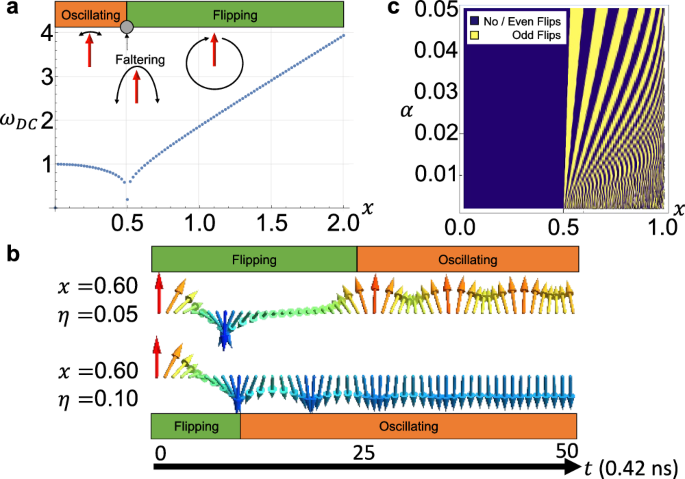
a Computed frequencies of oscillating (x < 0.5), faltering (x = 0.5), and flipping modes (x > 0.5) under DC current without damping in varying x = σ/K. b Dynamics of magnetization at x = 0.6, α = 0.05 (lower) and x = 0.6, α = 0.1 (upper) in time. Chromatically, the red indicates +z, the green indicates in-plane, and the blue indicates −z directions of magnetization. The direction inward of the paper is the y direction. c A 2D phase diagram of the final states in varying x and α. The dark blue indicates the even-flipped final state, and the yellow indicates the odd-flipped final state.
When damping α is introduced under DC current, the magnetization eventually attains an equilibrium state. For x ≥ 1, the equilibrium state aligns with the y-axis, so the spin-flip is absent. However, since two equilibrium states exist for x < 1, the selection between them occurs, which can flip the spin. The selection is determined by both x and α. Figure 2b displays two examples of dynamics leading to an even-flipped (x = 0.6, α = 0.05) and odd-flipped (x = 0.6, α = 0.1) final state, respectively. The magnetization in the even-flipped state stays in +z half-space, while that in the odd-flipped state stays in −z half-space. In both examples, owing to the damping effect, the crossover from the flipping to the oscillating mode occurs after a specific time τc. In Fig. 2b, for the former, after τc ≈ 10.8 ns, while for the latter, τc ≈ 4.2 ns. Empirically, we find that τc ∝ e4.53xα−1 for small α (see Supplementary Note 1). These show that the variation in τc caused by the interplay of x and α serves as a determining factor for the final state.
We further delve into the relation of the final state with x and α by a 2D phase diagram in Fig. 2c. When x < 1/2, exclusively the even-flipped final state manifests, whereas for x ≥ 1/2, both odd-flipped and even-flipped states emerge, forming a fan-like configuration. It should be noted that the fan-like configuration is not clear in α < 0.01 due to the resolution. The exclusive appearance of an even-flipped state for x < 1/2 is due to the absence of spin-flip in the oscillating mode. However, in the case of x ≥ 1/2, the spin-flip can occur multiple times before the crossover from the flipping to the oscillating modes takes place. If the crossover time exceeds half of the flipping mode period, the spin flips to −z half space. With a longer crossover time surpassing a full flipping mode period, the spin flips twice, returning to +z half space. By extending the crossover time further, the spin flips repeatedly. Even (odd) numbers of spin-flip lead to an even-flipped (odd-flipped) final state, giving rise to the distinctive fan-like feature in x ≥ 1/2. This pattern persists until x = 1, where the equilibrium state converges to the y-axis.
Magnetization dynamics under AC current
Based on the above results, we here explore the magnetization dynamics under AC current, which is given by (sigma (t)=sigma sin ({omega }_{{rm{AC}}}t+delta )) for t ≥ 0 and σ(t) = 0 for t < 0. ωAC is the driving frequency, and δ is the initial phase of AC current. The initial state of the magnetization is again aligned with +z-axis. Owing to the damping α, the relative strength of SOT x, and driving frequency ωAC, the initial state overcomes the irregular dynamics and transits to the final states after some time. We identify three distinct final states in Fig. 3a: adiabatic, resonating, and chaotic states. Both adiabatic and resonating states are the steady states coming after the decay of the initial state. At each time t, σ(t) determines an equilibrium state, as shown in Fig. 1b. The adiabatic state denotes that the magnetization mostly adheres to the equilibrium state at each time. The resonating state denotes that the magnetization dynamics are periodic but detach from the equilibrium state at each time. On the other hand, the chaotic state evolved from the initial state, retaining its irregularity, in which the magnetization never has a periodic motion.
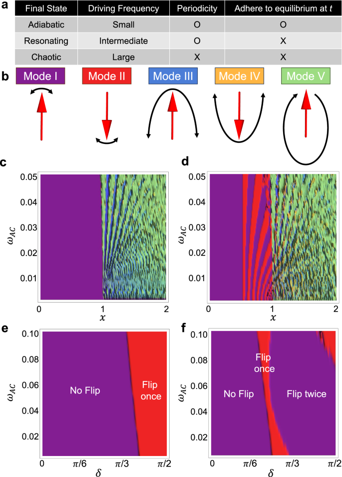
a The classification and comparison of final states. The final states transit with the driving frequency of AC, from adiabatic to resonating and to chaotic state in sequence. While adiabatic and resonating states have periodicity, chaotic state does not. While adiabatic state adheres to the equilibrium state at each t, others do not. b Schematics of distinct AC adiabatic modes after decay. c and d 2D phase diagrams of adiabatic modes in x and ωAC with α = 0.03, at (c) δ = 0 and (d) δ = π/2. e and f 2D phase diagrams of adiabatic modes in δ and ωAC at (e) x = 0.6 and (f) x = 0.8. The violet denotes Mode I, the red denotes Mode II, the blue denotes Mode III, the yellow denotes Mode IV and the green denotes Mode V.
We primarily observe the adiabatic states for low-frequency or strong damping regimes. We observe five distinct modes in the adiabatic states: (I) an even-flipped oscillating mode, (II) an odd-flipped oscillating mode, (III) an even-flipped faltering mode, (IV) an odd-flipped faltering mode, and (V) a periodically flipping mode. These modes are depicted in Fig. 3b. The even-flipped (odd-flipped) oscillating mode or Mode I (II) is the oscillation of magnetization within +z (−z) half space. The even-flipped (odd-flipped) faltering mode or Mode III (IV) is the repeated faltering of magnetization between xy-plane and +z (−z) half space. The periodic flipping mode or Mode V is the repeated magnetization flip. Notably, Modes I and II (or III and IV) are almost identical but differ in the number of spin flips before decaying to the adiabatic state. Only Mode V shows the continuous spin flip in time in its adiabatic state. As one can expect from their names, the adiabatic modes originate from DC modes. Modes I and II come from oscillating mode, Modes III and IV come from the faltering mode, and Mode V comes from the flipping mode.
The modes are chosen by the interplay of x, ωAC, δ, and α. Both x and ωAC underscore their importance after decaying to adiabatic states, while δ and α play a pivotal role during the decay process. Primary investigation is performed by phase diagrams for the modes in x and ωAC at α = 0.03 with different δ presented in Fig. 3c, d. For x < 1, Modes I and II appear, while for x ≥ 1, Modes III, IV, and V manifest. The repeated spin flip in the adiabatic state, therefore, can only occur for x≥1. Since the necessary condition for spin flip is that the magnetization reaches the xy-plane, the equilibrium state must reach at ± y axis at some time t. For x < 1, as the equilibrium position does not reach the y-axis at any time, the magnetization oscillates within either +z or −z half space. For x ≥ 1, however, as the equilibrium reaches the y-axis, the magnetization either falters on the xy-plane or flips its position between +z and −z half spaces periodically.
ωAC also plays a role in determining the modes. Primarily, ωAC chooses the faltering and flipping modes when x ≥ 1, since it determines the time duration τy that the equilibrium state at each time stays at the y-axis. One can obtain the duration by finding the maximum τy satisfying σ(t) ≥ 1 in t ∈ [t0, t0 + τy]. In the case of sinusoidal σ(t), this can be expressed as ({tau }_{y}=frac{1}{{omega }_{{rm{AC}}}}(pi -2zeta )), where (zeta =arcsin (1/x)in (0,pi /2]). For τy, as the equilibrium state is at the y-axis, the magnetization modulates near the y-axis. After τy, the equilibrium position is divided again and deviates away from the y-axis. Then, depending on its modulated position, the magnetization chooses one of the equilibrium states, which leads to either faltering or flipping modes. Additionally, the window of x for every mode at higher ωAC is opened up wider than that at lower ωAC, showing the fan-like feature in Fig. 3c, d. Unlike the faltering mode under DC current, the window of Modes III and IV, originating from the faltering mode, expands to the finite range of x. Lastly, it is noteworthy that the phase of ωAC = 0 in Fig. 3d is the same as the phase in α = 0.03 line of Fig. 2d. This substantiates that adiabatic modes can be derived from DC modes.
On the other hand, δ acts as a switch to turn on the spin-flip during the decay process to adiabatic states. Specifically, comparing Fig. 3b to c, Modes II and IV barely appear when δ = 0, which means that the spin-flip is turned off near δ = 0. This happens because the average of σ(t) during the decay time is small, so the spin cannot flip before decaying the adiabatic state. This can be supported by Fig. 3e, f. In Fig. 3e, we present phase diagrams for the modes in δ and ωAC at x = 0.6. The transition from Modes I to II occurs once during the increase of δ. This happens because the spin-flip is turned on by finite δ. Increasing x, the spin flips more times, just as in the DC case, so the repeated transition between Modes I and II can also be observed in Fig. 3f. We should note that the increase of α reduces the decay time. The above arguments also hold for the triangular wave instead of the sinusoidal wave (see Supplementary Notes 2 and 3).
We move on to high-ωAC and low-α regimes to investigate ferromagnetic magnetoresonance (FMR). One could expect that the resonance frequency is closely related to the frequencies ωDC in Fig. 2a. In fact, when ωAC approaches ωDC, the oscillating amplitude becomes larger, and eventually, the adiabatic state changes to the resonating state and to the chaotic state sequentially. By checking the final state after t ~ 0.25 ms (6 × 10⁵ unit times), we present 2D phase diagrams in ωAC and α at x = 0.3 and 0.7 in Fig. 4a. Both diagrams show similar behavior. It begins with the adiabatic state at low frequencies, confronts the transition to the resonating state, and reaches the chaotic state at a certain range of ωAC. For x = 0.7, the window of chaotic states is opened up widely as SOT becomes large. We can find the transition from adiabatic to chaotic states for x > 1 as well.
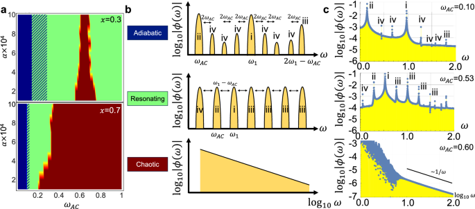
a 2D phase diagrams of the final states in ωAC and α. The adiabatic state is in dark blue, the resonating state is in green, and the chaotic state is in dark red. The top panel is at x = 0.3 and the bottom panel is at x = 0.7. b The schematics of change in Fourier transform for each state. c The corresponding examples to each state of b at x = 0.3 and α = 0.
We further illuminate the transition of states by the Fourier transform. The transition is illustrated in Fig. 4b, where the change in ∣ϕ(ω)∣ by ωAC is schematically presented. Here, ϕ(ω) corresponds to the Fourier transform of azimuthal angle ϕ(t) from t = 0 to t = 0.21 ms (5 × 10⁵ unit times). Figure 4c showcases representative examples of Fourier transforms at x = 0.3 and α = 0. For adiabatic and resonating states, four distinct peaks are observed in the top panels: (i) a main peak at ω1 derived from ωDC, (ii) another main peak driven by AC at ω2 = ωAC, (iii) induced peaks from (i) and (ii) at ω3 = ω1 + n(ω1−ωAC), and iv) subpeaks at ω4 = ∣ω1,2,3 ± 2nωAC∣ ((nin {mathbb{N}})). Notably, Peaks (i) and (iii) are strong near t = 0 while Peaks (ii) and (iv) gain intensity near the final state (see Supplementary Note 4). This means that Peaks (i) and (iii) are related to the decay process, while Peaks (ii) and (iv) are related to the stable state after decaying. Increasing ωAC to the higher frequency, the change only occurs to the distance between peaks, as the frequency of Peak (i) decreases and that of Peak (ii) increases. Thus, adiabatic and resonating states are indistinguishable solely by Fourier transform. This is substantiated by the phase diagrams in Fig. 4a, where the transition from adiabatic and resonating states is not distinctly delineated. This behavior is consistent for all modes in Fig. 3b. Near the chaotic state, the peaks form an array in a period of ωAC−ω1, as shown in the middle panels. As ωAC increases more, chaos sets in, destroying all peaks and being ϕ(ω) ∝ 1/ω, as shown in the bottom panels. This behavior does not change, although the range of time is elongated to t > 0.21 ms.
Magnetization dynamics under a magnetic field
In this section, we discuss the magnetization dynamics under a magnetic field. Let us consider the following experimental situation. Originally, the magnetization is at the z-axis, and we adiabatically apply a magnetic field (overrightarrow{B}) to the system at t → −∞. Then, the magnetization moves to a new equilibrium state at t = 0. The current is introduced at t = 0, inducing the magnetization dynamics. The Lagrangian describing the system is now ({mathcal{L}}={{mathcal{L}}}_{{rm {B}}}-{V}_{{rm {A}}}-{V}_{{rm {S}}}^{{prime} }), where ({V}_{{rm {S}}}^{{prime} }=-gamma overrightarrow{m}cdot (overrightarrow{sigma }+overrightarrow{B})). When (overrightarrow{B}) is in-plane ( + x-axis), the initial position is at θ(0) = π/2 and (phi (0)=arcsin (B/K)). As the equilibrium position is just rotating around the z-axis, all modes can be found for both AC and DC cases. For DC dampingless case, we find the transition between oscillating and flipping modes around (sqrt{{(K/2)}^{2}-{B}^{2}}). For the AC case with cosine wave ωAC = 0.03 and α = 0.03, we find Mode I at x = 0.4, Mode II at x = 0.7, Mode III at x = 1.05, Mode IV at x = 1.31, and Mode V at x = 1.1 at B = 0.01, 0.02 (see the “Methods” section).
The nontrivial case is the out-of-plane direction. We here take the simplest case of (overrightarrow{B}=B(0,0,1)) into account. For m = γ = 1, the equation of motion is
For the DC current without damping, we find the oscillating and flipping modes. We investigate B = −0.10, −0.05, −0.01, 0.01, 0.05, 0.1, 0.2, 0.3, 0.4, and 0.5 by numerical simulation. The transition from oscillating and flipping modes occurs around x = 0.409, 0.453, 0.491, 0.51, 0.55, 0.6, 0.7, 0.8, 0.9 and 1.0, which are ~K/2 + B. The faltering mode is not observed since it needs fine-tuning. When damping is introduced α = 0.03, we find that the magnetization flip is enhanced under the −z field while prevented under the +z field. We investigate the final states at B = ± 0.001, ± 0.01, ± 0.02, ± 0.03, ± 0.05, ± 0.1 at x = 0.63, 0.7, 0.83. This is the parameter range where the flipping modes occur at t = 0. For the +z field, The magnetization flip occurs up to B = 0.03 at x = 0.63 and up to B = 0.02 at x = 0.7 and 0.83. The magnetization flips only under a weak magnetic field. This indicates that the magnetization flip is prevented. For the −z-field, the magnetization flips everywhere except B = −0.02 to −0.05 at x = 0.63. Considering that the exceptions come from additional flips, the magnetization flip is enhanced.
This happens similarly in the AC adiabatic modes. We apply a cosine current with ωAC = 0.03 and α = 0.03 and investigate the modes at B = ±0.001, ±0.005, ±0.01, ±0.02, ±0.10 at x = 0.4, 0.7, 1.05, 1.1, 1.31. We summarize the results in Table 1. Without a magnetic field, x = 0.4 shows Mode I, x = 0.7 shows Mode II, x = 1.05 shows Mode III, x = 1.31 shows Mode IV, and x = 1.1 shows Mode V. Increasing the field strength to the +z direction, Modes IV and V change to Mode III, and Modes II and III change to Mode I. For B = 0.01, only Mode I can be observed up to x = 2. Modes II and IV are the magnetization flip during the decay process, and Mode V is the repeated magnetization flip at the adiabatic state. Therefore, the magnetization flip is prevented by the +z field. However, for the −z direction, every mode changes to Mode II. Even Mode I at x = 0.4 changes to Mode II beyond B = −0.01. The magnetization flip is enhanced by the −z field. Lastly, the chaotic state appears for high ωAC even under a magnetic field.
The reason for the phenomenon is that the magnetic field changes the equilibrium position for x ≥ 1. In the “Methods” section, we acquire the deviation of equilibrium position by a small field. For x > 1, at which the current strength is large, the angle between the xy-plane and the equilibrium state is ~B/(σ−K). (Note that for x = 1, the angle is ~(2B)1/3.) As we mentioned in the previous sections, the necessary condition of magnetization flip is that the equilibrium position reaches the xy-plane. Thus, as the angle grows by increasing the +z field, the equilibrium position does not reach the xy-plane, so the magnetization flip is prevented. However, by increasing the −z field, the equilibrium position reaches the xy-plane with less x, so the magnetization flip is enhanced.
Discussion
We address here the typical values of parameters in realistic systems. The typical value of ferromagnetic anisotropy is 1−10 μeV/atom27, that of the current density in the experiments is ~107 A cm−2, and that of the itinerant spin polarization by Rashba–Edelstein effect is estimated at about 10−4ℏ per unit cell46. The typical value of the Gilbert damping constant is ~10−3−10−2 47, and that of the unit of AC frequency is estimated at about 1−10 GHz. The unit of magnetic field is ~1 μB T.
Although we mainly discuss the TI–FM heterostructure due to its high efficiency, our work can be applied to the general systems with strong Rashba spin–orbit coupling, i.e., heavy metal–FM heterostructures. This is because the assumption underlying our work is only that the current carries finite spin due to the Rashba–Edelstein Effect. We here list some candidate systems. For TI–FM heterostructure, (Bi0.5Sb0.5)2Te3/(Cr0.08Bi0.54Sb0.38)2Te323, Bi2Se3/Ni81Fe1924, Bi2Se3/CoTb25, Bi2Se3/NiFe26, and (Bi1−xSbx)2Te3/Cr2Ge2Te627. For heavy metal–FM heterostructure, Pt/Co48,49,50, AuxPt1−x/Co51, and Ta/CoFeB/MgO52,53.
So far, we discuss the magnetization dynamics at the interface of TI–FM heterostructure. We emphasize that our work systematically classifies the modes of magnetization dynamics and describes the mechanism and condition for the spin-flip. Under DC current, we observe the oscillating and flipping modes without damping, which is determined by the relative strength of anisotropy and SOT. With damping, the number of spin flips is determined by the duration of the crossover from flipping to the oscillating mode. Under AC current, we observe five distinct modes in the low-frequency regime and their evolution to the resonating and chaotic states in the high-frequency regime. We also discuss the effect of the magnetic field on the spin dynamics. Our work offers insights into spin control by spin–orbit coupling, underscoring the practical aspects of the world of spintronics.
Methods
Computational method
The numerical computation of spin dynamics from Eqs. (4) and (5) is performed by using the “NDSolve” function of Mathematica. The initial condition is θ(0) = π/2 and ϕ(0) = 0 in the absence of magnetic field and in the presence of out-of-plane magnetic field, θ(0) = π/2 and (phi (0)=arcsin (B/K)) for the in-plane magnetic field. We used an automatic solver. AccuracyGoal and PrecisionGoal are automatic, which are set to be a half of Machineprecision 15.9546.
The induction of LLG equation
Let us take the y-axis as the polar axis. Then, the magnetization is
and (overrightarrow{sigma }=sigma (0,1,0)). The initial condition is given by θ = π/2, ϕ = 0. There are three terms in the Lagrangian density:
The Lagrangian density is
The Rayleigh dissipation function is
Here, ({partial }_{t}overrightarrow{m}=m(dot{theta }hat{theta }+sin theta dot{phi }hat{phi }).)
The equations of motion is
Note that
Thus,
Tidy up,
Also,
Let m = γ = 1, then ηγ = η × 1 = α. The equation becomes
Note that this holds though σ is time-dependent. Divide the first equation by (sin theta),
Let us compare this to the LLG equation. Given that the Lagrangian is (L[overrightarrow{m},{partial }_{t}overrightarrow{m}]=T-V), we can get LLG equation by the following equation of motion.
Then,
where (overrightarrow{H}=-frac{partial V[overrightarrow{m}]}{partial overrightarrow{m}}) is the effective field, and the Gilbert damping constant α = γη. With γη = α and γ = m = 1,
The time derivative of (overrightarrow{m}) is ((0,dot{theta },sin theta dot{phi })) in ((hat{r},hat{theta },hat{phi })) basis. The effective field is
In the spherical basis, one can find
Also,
Thus, we have
This is just the same as Eq. (20) by changing θ → −θ, ϕ → −ϕ.
The equilibrium state under a magnetic field
First, we obtain the equilibrium state under a magnetic field. (overrightarrow{sigma }=sigma (0,1,0),overrightarrow{B}=B(0,0,1)), and (overrightarrow{m}=m(sin theta cos phi ,sin theta sin phi ,cos theta )), where σ > 0, m > 0, B > 0. Note that here the z-axis is the polar axis. We use perturbation to obtain the equilibrium state.
We acquire the equilibrium state as follows. The potential energy is given by
For simplicity, we let m = γ = 1 at the last line. The derivative gives
When x = σ/K > 1 and B = 0, the ground state is θ0 = π/2, ϕ0 = π/2. Thus, we let θ = θ0 + δθ(B), ϕ = ϕ0 + δϕ(B). Then,
By letting (cos delta theta ,cos delta phi ,approx 1) and (sin delta theta ,sin delta phi approx delta theta), we have
The zeroth-order of B terms are
The first-order of B terms are
From the second equation, δϕ = 0. Then,
Thus, (delta theta =-frac{B}{sigma -K}, < ,0), so the equilibrium position does not reach + y-axis and xy-plane.
For x < 1, the ground state is ({theta }_{0}=arcsin x) and ϕ0 = ϕ/2. There are two θ0 in [0, π], such that (cos {theta }_{0}=pm sqrt{1-{x}^{2}}). From Eq. (34), both of θ0 gives
Thus, δϕ = 0 and
At x = 1, we expand Eq. (30) up to the third order of δθ and δϕ at θ0 = ϕ0 = π/2. Then,
δϕ = 0 is a physical solution of the second equation. Therefore, x = 1,
The lowest order of B in δθ is −(2B)1/3. The equilibrium position does not reach the xy-plane.
The LLG equation under a magnetic field
Let us build the LLG equation under a magnetic field here. Let us take the y-axis as the polar axis. Then the magnetization is
and (overrightarrow{sigma }=sigma (0,1,0),overrightarrow{B}=B(0,0,1)). The initial condition is given by θ = π/2, ϕ = 0. We let γ = m = 1. The terms we have now are
The Lagrangian is
The Rayleigh dissipation function is
The equations of motion are
Note that
Thus,
Tidy up,
Note that ηγ = α and γ = 1,
Let us consider the in-plane field (overrightarrow{B}=B(1,0,0)). The Lagrangian is composed of:
The equations of motion are now straightforward.
Thus,
Also, γ = 1 gives γη = η = α,
The initial condition now is θ(0) = π/2 and (phi =arcsin (B/K)).
For DC dampingless case, with B = 0.01, 0.02, 0.03, 0.04, and 0.05. We find the transition of oscillating and flipping modes around x ∈ [x0, x0 + 0.005], where ({x}_{0}=sqrt{{(K/2)}^{2}-{B}^{2}}). For the AC case with cosine function at ωAC = 0.03, B = 0.01, 0.02 and α = 0.03, we find Mode I at x = 0.4, Mode II at x = 0.7, Mode III at x = 1.05, Mode V at x = 1.1, and Mode IV at x = 1.31. The physics does not change much under the in-plane magnetic field.


Responses