Urban residential clustering and mobility of ethnic groups: impact of fertility

Humanity increasingly lives in urban settings, characterised by fertility decline and multiethnic composition. Quantifying the levels of residential segregation in urban areas and their associations with the population growth and fertility are key for understanding and predicting demographic changes. Several conceptual and methodological paradigms exist for studying socioeconomic heterogeneities observed in spatial distributions of populations. Important approaches include the formulation of spatial indices, recognizing the multiple dimensions, cartographic projections, modelling of the underlying dynamics, and the inclusion of demographic factors^{1,2,3,4,5,6,7}. Much of this research has focused on urban populations in the United States and major European countries, especially ones with a long history of immigration and settlement^8,9,10,11. Both from the viewpoint of research and policy making, segregation is largely considered as a negative outcome at the societal level^12,13.

In this work, we propose to quantify segregation and population dynamics using the general ideas of scaling laws which have been widely used to characterise how macrolevel quantities of cities, such as urban GDP and productivity, vary with population size¹⁴. The types of scaling relations have been argued to generally differ depending upon whether the quantity is related to social interactions or to infrastructures^15,16. Recent studies have also examined temporal scaling laws in which a relevant quantity for a city is studied as a function of its growing population and, therefore, is used to quantify the historical evolution^17,18,19. Apart from such allometric scaling, the notions of fractality and power-laws have been long-investigated in urban systems. The latter approach has also been used to model the dynamical nature of city growth including intra- and inter-urban migration^16,20,21.

We begin with a model for the propensity of ethnic minority groups to inhabit spatially contiguous areas. We modify a null model²² for spatial distribution of populations by assuming that the number of individuals of a group in an area would scale as the group population in the neighbouring areas. Thus the model provides a measure of spatial clustering that has been conceived as one of the dimensions of segregation^3,23. We additionally include a set of socioeconomic variables that could independently influence the spatial clustering of minorities in the model. Next, we use similar models for studying migration flows of groups to understand how spatial clustering may be reinforced over time. The models employ microlevel register data from Finland with detailed socioeconomic, demographic and geographic information, enabling us to compare the spatial and temporal clustering of different ethnic groups residing in the capital region. We focus on the capital region, since we are interested in urban segregation, and since other regions of Finland have too low proportions of different ethnic groups to warrant a detailed analysis.

Compared to North America and most other European countries, the history of international migration to Finland can be considered rather recent²⁴. The proportion of the population with a migrant background was less than one percent in 1990 and is currently around 9 percent. The primary countries of origin of migrants to Finland have been the European countries, especially Sweden, Russia and Estonia. Additionally, immigration took place through refugee waves at different points of time. The topic of social segregation of ethnic minorities has been well studied for the Finnish population owing to the availability of microlevel data from population registers. Past research included descriptive studies, measurement of segregation indices, integration efforts, and impact of policies related to job markets and housing, among other aspects^24,25,26,27. Notably, the municipalities in the capital region including Helsinki and the neighbouring areas are known to have official strong desegregation policies^28,29. By the end of 2019, one-half of those with a migrant background in Finland resided in the Greater Helsinki metropolitan region. Also, foreign language speakers accounted for over 70% of the net migration into the region³⁰.

Spatial clustering

As a starting point for a model to quantify clustering we began with the framework presented by Louf and Barthelemy²². The authors considered a null model for the distribution of the population of different groups over the area units in a city that is unsegregated. Adopting the framework to the current problem, let n_i,g and n_i denote the population belonging to a group g and the total population in an area unit i of the Greater Helsinki (GH) region measured at any point of time, respectively. Here, g represents the groups enumerated in Fig. 1, and additionally the native Finnish and Swedish speakers (see the “Methods”). An area unit i belongs to a square grid with respect to which the residential locations of people are available in the dataset. Given that the total population of group g is N_g, such that ∑_gN_g = N_GH = ∑_in_i, where N_GH is the total population in GH, and with n_i,g < < n_i, the null model would predict the following expectation value for populations,

However, in reality, several socioeconomic factors are expected to influence the distribution of the population of different groups. One such factor is the tendency to cluster based on language or ethnicity, which is a key aspect we aim to measure. This also encompasses the propensity for close kin to reside in spatial proximity^31,32. We assume that the population of a group in a location i could be predicted by the population of people from similar ethnicity in the adjoining areas. We quantify this effect by considering that the expectation value in the above model is modified by a prefactor ({widetilde{n}}_{i,g}^{{beta }_{s}}), where ({widetilde{n}}_{i,g}) is the population of individuals belonging to group g per unit area in a neighbourhood ({{mathcal{N}}}_{i}) and the exponent β_s is the measure of clustering. To measure β_s for different groups we formulated this as separate regression model for each group as follows

where ϵ_i,g is a normally distributed error with zero mean. To calculate ({widetilde{n}}_{i,g}), we chose ({{mathcal{N}}}_{i}) as the set of eight units in the Moore neighbourhood around the area unit i. We refer to Eq. (2) as the ‘base model’.

a The region of Greater Helsinki including the capital city of Finland, Helsinki, and sixteen other municipal regions. The municipalities surrounding Greater Helsinki are shown in a lighter shade. The grid is constituted by 1 km² cells from which data on residential locations is available. The population is predominantly composed of native Finnish speakers. The heat map corresponds to the population of different socioethnic groups in 2019 including individuals with an international-migrant background as well as the Swedish speakers native to Finland. Finland is officially a bilingual country. Around 86 percent of the population have Finnish as their registered maternal tongue and five percent have Swedish. Swedish speakers thus constitute a linguistic minority in Finland with several own cultural traditions, media outlets, and schools. b The population of different groups in Greater Helsinki are shown corresponding to the different years. The group `Africa’ includes countries in sub-Saharan Africa. c The aggregated migration flows during the period of 1988–2020 for the groups are shown. The flows include both international migration and internal migration, or individuals entering from or leaving for other regions of Finland. The net flows (difference between the total incoming and total outgoing flows) are denoted in grey. In 1990, there were roughly 80 thousand native Swedish speaking natives in Greater Helsinki, and by 2019 their population marginally dropped. In this period, the population of the native Finnish speakers grew by 20% to around 1.2 million. For these two groups the flows in either directions aggregated over the period were rather balanced—around 0.6 million for Finnish speakers and 30 thousand Swedish speakers.

Full size image

Although, we started from a null model Louf and Barthelemy²², the variable n_i can be alternately thought of as a proxy for factors that would typically influence the growth of population at the i-th location. Previously, Jones et al.^33,34 presented a similar approach for structuring models around the expectation of counts within the categories in the contexts of assimilation and segregation^33,34. Studies using different modelling schemes have also considered measurement of segregation that is conditional or controlled with respect to different observed characteristics of groups that simultaneously influence the clustering of populations^35,36. Our approach is similar to the earlier works that have included additional explanatory variables in the models to account for the characteristics of individuals, groups, and locations^5,37,38.

Within the current scheme, we add the following three variables:

1. (a)

   Income is a factor understood to be intricately related to the dynamics of residential segregation in cities as detailed by, for example, Bayer et al.⁵. The mean income of individuals at a location could reflect the housing prices. However, income of individuals and groups, in general, can both be a cause and an outcome of the sorting process of groups into different locations^39,40. Here, we include <m>_i, the average income in an area unit i that was calculated from summing of the yearly disposable incomes of all the individuals in the unit irrespective of group affiliations. By including this variable in the model we expect β_s to capture the aspect of clustering that is unrelated to income^5,41.

2. (b)

   In their work Massey and Denton³ introduced “centralization” as one of the dimensions of segregation to explain possible tendency in an immigrant population to reside near the centre of a city that was tacitly assumed to be the hub of economic activity⁴². We take this possibility into consideration via the variable d_cen,i, the distance between an area unit i and the centre of GH. Although the capital region is generally not considered to be mono-centric, the central location does have substantially larger share of the population and employments^43,44.

3. (c)

   Previous studies have also discussed linkages between residential and workplace segregation. Individuals who are employed in the same workplace are prone to also reside near each other, and vice versa^5,38,45. Therefore, we expect people with similar skills to also cluster in terms of residential locations irrespective of the their ethnic affiliations. We take this aspect into account by including the variable D_KL(P_g,i|| Q_i), which is the Kullback-Leibler (KL) distance measured between the empirical distributions of socioeconomic statuses P_g,i and Q_i. The dataset contains information on the socioeconomic statuses of individuals, for instance, whether a person is self-employed or an upper-level employee. A complete list is provided in the Supplementary Fig. 2. Using this information we calculated P_g,i for people belonging to a group g residing at location i. Similarly, we calculated Q_i taking into account all the people residing in i and in the neighbourhood ({{mathcal{N}}}_{i}). A small KL distance implies a high similarity between the socioeconomic profiles of people from group g and the rest of the population residing in and around the area, and therefore, could independently explain a large value of n_i,g.

With the inclusion of the above variables the ‘full model’ reads as follows:

Here, we did not control for variables that have direct functional dependence on age, sex and education of the residents, which were considered in some of the previous studies^5,35,36,45. We assumed that the possible variation in n_i,g due to the latter variables were accounted for by the income and the socioeconomic status. Additionally, we assumed that there were no omitted variables that were significantly correlated with (log {n}_{i}), in particular. We used ordinary least squares (OLS) to evaluate the coefficients in the model separately for the groups using data from the year 2019. We checked the level of collinearity among the explanatory variables using the variance inflation factor (VIF). Except for one instance ((log {d}_{{rm{cen}},i}) for Scandinavia) all the variables in the full model for all the groups had VIF less than the commonly accepted cutoff 5.0 (see Supplementary Fig. 6). There is, however, a level of complexity involved in estimating the coefficient of ({widetilde{n}}_{i,g}). See the “Methods” for details and relative fit indices for the null, the base, and the full model.

The coefficient quantifying spatial clustering (Fig. 2a) obtained from the full model containing all the explanatory variables was generally lower than the one obtained from the more restricted base the model. The reductions were substantial especially for the populations corresponding to high income-countries and Somalia. The coefficient was found to range between zero and 0.5, and was highest for the native Swedish-speaking population. The spatial clustering as measured using the base model could reflect two distinct processes unravelling over longer periods of time, and namely, fertility and migration. As a measure of fertility for the cross-sectional data we used the child to woman ratio (CWR) for the different groups. It was calculated as the ratio between the number of children under five and the number of women aged between 15 and 49, considering the individuals in the population register during 2019. In general, the clustering was found to increase with the fertility of the groups (Fig. 2b). Given two groups with the same population sizes, the one with the higher child-woman ratio would tend to have larger families, and therefore would show a higher clustering in space. The base or the full models were not strictly applicable to the case of native the Finnish speakers given n_i,g ≃ n_i, in general. For the sake of completeness we measured the clustering in the latter case, and as expected, β_s was observed to be negligibly small.

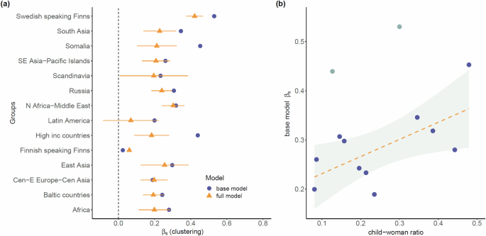
a The measure of clustering is plotted for the different groups. In general, the introduction of additional explanatory variables deflates the clustering as can be observed by comparing the results from the base and the full models. The error bars for the full model depict 95% confidence intervals. The bars for the base model are omitted for clarity. b The clustering is plotted against the child-woman ratio which is a cross-sectional measure of fertility of groups. Considering the groups Swedish-speaking Finns and high income-countries as outliers, the dashed line has a slope of 0.35 (p < 0.05, R² = 0.43). See the Supplementary Fig. 16 for the characterization of outliers. This plot suggests that part of the variability in clustering could be explained by differences in fertility.

Full size image

Next, we show the coefficients (exponents) corresponding to the other explanatory variables. In Fig. 3a we show the dependence on the total population in an area unit, which we have interpreted as the general attractiveness of an area. For the groups, in general, β_n > 0 which implies that the higher the total population in an area unit, the higher is the group’s population. For some groups, such as North African-Middle Eastern migrant origins, the dependence was strongest, while it was weakest for Swedish-speaking Finns. The Fig. 3b shows β_m ≤ 0, which implies inverse relationship between the group population and the mean income at the locations. While this effect was pronounced for a group like migrants with Somalia as the country of origin, for groups like high income-countries, Swedish-speaking Finns, Scandinavia, and Latin America the effect was almost absent. The Fig. 3c also shows an inverse relation with the distance from the centre of Helsinki. The latter relationship appeared to be weak as β_cen was non-significant in many of the cases. The population appeared to decrease fastest with the distance from the centre for the high income-countries. In Fig. 3d we show − β_KL, which quantifies the tendency of individuals to reside beside other individuals of similar socioeconomic status.

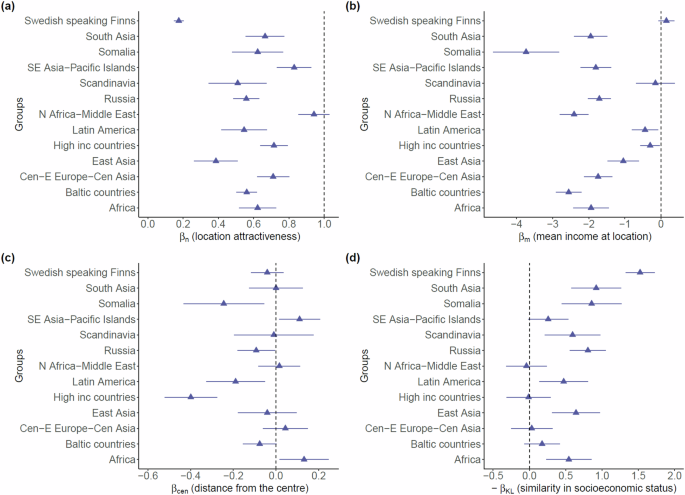
The relevance of the variables within the model are the following: (a) location attractiveness, (b) mean income at the location, (c) distance from the city centre, and (d) similarity in socioeconomic status.

Full size image

Migration and clustering

We compared the changes in population for the different groups in different area units due to migration within the Greater Helsinki region. Although the overall population growth of ethnic minorities could be largely attributed to migration from outside Greater Helsinki, the local changes are dominated by moves within the metropolitan area. This was evidenced by comparing the magnitudes of the intra-regional migration flows and other types of flows (combining emigration, immigration, and flows from or to other regions of Finland), and examining the ratio between those two quantities (see Supplementary Fig. 10). Similar to the case of the population distribution, we assumed a null model for the yearly flow of a group at any area unit i:

where M denotes whether the flow is incoming or outgoing, F_i,g is the inflow or outflow in the area unit i for group g, F_i is the total flow in area unit i, F_g is the total flow for the group g, and F_GH is the aggregated flow for the entire region. Note, that the condition ∑_iF_i = F_GH = ∑_gF_g holds separately for inflow and outflow. In addition, the condition ({F}_{{rm{GH}}}^{{rm{in}}}) = ({F}_{{rm{GH}}}^{{rm{out}}}) was approximately satisfied depending on the filtering and the quality of data.

For the inflows we modified the null model in the following way. First, we used the additional variable ({n}_{i,g}) to quantify the ‘presence’ of a group within the area unit. Second, as the migration was intra-region we considered the possible presence of social gravity whereby people would tend to relocate to nearby locations¹⁶. Ideally, a model on gravity would imply studying the flows between pairs of locations, but in the current model involving just focal locations, we included the total outflow ({widetilde{F}}_{i,g}^{{rm{(out)}}}) of the group from the neighbourhood ({{mathcal{N}}}_{i}) as an explanatory variable. Also note that in case of a gravity model we would need to deal with noisier and sparser group-level flows resulting in poorer model fits. Therefore, the inflow model in terms of aggregated flows was specified as,

where (log {n}_{i,g,tau }) is the population of group g in the year τ, and the ({mathcal{F}})’s are flows aggregated over a period between τ and τ + Δ. The latter aggregation was done to reduce the noise in the yearly flows F. The coefficient α_F is expected to account for the population-level factors influencing the flows to an area unit, and α_p is to account for the presence of the group g. The coefficient α_s should quantify the tendency to relocate between nearby locations. For the outflows emanating from an area unit we solely considered the attributes of the focal unit:

The Eqs. (5), (6) constituted as our base models for migration within the region. Further, we extended these models by including the centralization variable d_cen,i and the average income in the area unit in the year τ,<m>_i;τ as explanatory variables. For brevity, we provide only the full model corresponding to the inflow:

We aggregated flows by summing the flows ({F}_{{tau }^{{prime} }}) in each year ({tau }^{{prime} }) which gave ({{mathcal{F}}}_{tau ,Delta }=mathop{sum }nolimits_{{tau }^{{prime} } = tau +1}^{tau +Delta }{F}_{{tau }^{{prime} }}), where τ ∈ {1995, 2000, 2005, 2010, 2015} and Δ = 5. While it was possible to run the regressions separately for each τ, we mean-centred the variables for each τ and then performed the regressions after pooling the data from different time windows. The mean-centreing enabled us to take into account the population growth that would have taken place over time in the area units. The VIFs for all the explanatory variables for all the groups were less than 5.0 (see Supplementary Fig. 13). Ten out of the thirteen groups that we investigated (not including the native Finnish speakers) had adjusted-R² for the inflow models in the range 0.4–0.8. The lower values for the rest three (for example, Scandinavians) could have resulted from smaller sample sizes. The outflow model in general had a higher explanatory power but with marginal difference between the base and the full model (see Figure 14 and Table V of the Supplementary Information for the fit indices). Finally, we combined the inflow and outflow models to arrive at the following general expression for the ratio of the inflow to the outflow across area units:

where, (Delta {alpha }_{p}={alpha }_{p}^{{rm{(in)}}}-{alpha }_{p}^{{rm{(out)}}}), (Delta {alpha }_{m}={alpha }_{m}^{{rm{(in)}}}-{alpha }_{m}^{{rm{(out)}}}), and (Delta {alpha }_{{rm{cen}}}={alpha }_{{rm{cen}}}^{{rm{(in)}}}-{alpha }_{{rm{cen}}}^{{rm{(out)}}}).

We investigated whether α_s, which captures the tendency to move locally could be associated to the the observed clustering in space (Fig. 4). First, we considered only the base models in which the variables were primarily geometric in nature. Treating the observation for Swedish-speaking Finns as an outlier, we were able to observe a significant association (slope) between β_s and α_s. Given that β_s was separately found to depend on the child-woman ratio, we examined β_s’s joint dependence on α_s and CWR (Table 1). With the base models we found β_s to significantly vary with both CWR and α_s (adj. R² = 0.88; F_2,8 = 39.04, p < 0.001). In case of the full models only the relationship to α_s remained significant (adj. R² = 0.73; F_2,9 = 16.16, p < 0.01).

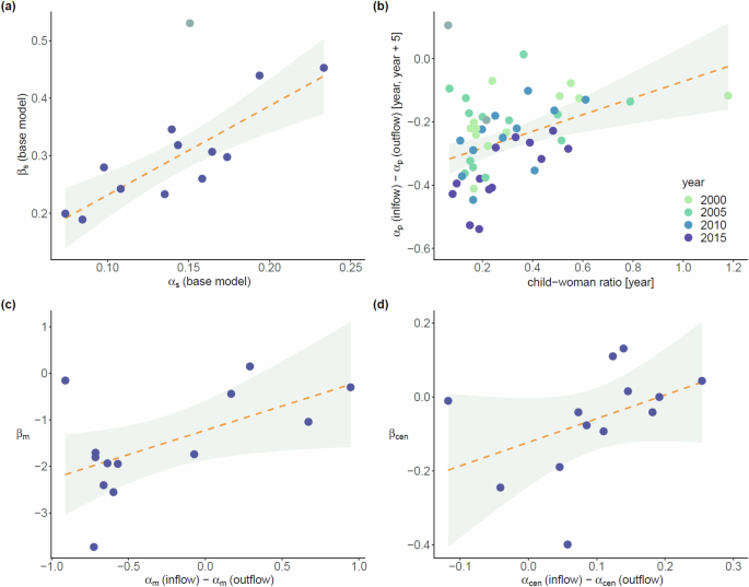
a Relationship between clustering (β_s) measured in the spatial base model and the coefficient (exponent) of neighbourhood outflows (α_s) in the inflow base model. The point corresponding to the Swedish-speaking Finns is considered as an outlier to a linear relationship and is shown in a lighter shade. The slope of the fitted line is 1.54 (p < 0.001, R² = 0.74). The shaded region is the 95% confidence interval. We show β_s‘s joint dependence on α_s and the CWR in Table 1. b The coefficient of group population, (Delta {alpha }_{p}={alpha }_{p}^{{rm{(in)}}}-{alpha }_{p}^{{rm{(out)}}}) in the model of inflow-outflow ratio is plotted against the child-woman ratio. The inflow and outflow coefficients are obtained from the base models. Each data point represents the regression coefficient corresponding to a group and a specific period over which the yearly flows were aggregated. While the CWR was calculated for the years (τ) as shown in the legend, the flows corresponded to [τ, τ + Δ] with Δ = 5. The dashed line has slope of 0.26 (p < 0.01, R² = 0.18). Note, in general, for all the groups ({alpha }_{p}^{{rm{(out)}}} ,>, {alpha }_{p}^{{rm{(in)}}}). Two of the data points (grey) were excluded from the regression fit (see Fig. 16 and Table VI of the Supplementary Information). Plots (c) and (d) illustrate the behaviour of the coefficients from the spatial full model against relevant coefficients in the inflow-outflow ratio. c Coefficient of the mean income at area unit β_m versus (Delta {alpha }_{m}={alpha }_{m}^{{rm{(in)}}}-{alpha }_{m}^{{rm{(out)}}}) (slope = 1.04, p < 0.05, R² = 0.32). d Coefficient of distance from the city centre β_cen versus (Delta {alpha }_{{rm{cen}}}={alpha }_{{rm{cen}}}^{{rm{(in)}}}-{alpha }_{{rm{cen}}}^{{rm{(out)}}}) (slope = 0.64, p > 0.1, R² = 0.18).

Full size image

In the premise of the base models we also checked for any association between the coefficient Δα_p and the CWR (Fig. 4b, also see Supplementary Table VI). Naively, the observed behaviour could indicate that the groups with higher fertility accumulate population from other areas over time. However, the vertical axis shows that for the groups Δα_p < 0 implying that the inflow to outflow ratio varies inversely with the local group population (density). Therefore, individuals irrespective of group affiliation would tend to migrate out over time from areas with higher concentration. Apparently, the rate at which the latter occurs is influenced by the overall CWR, which is likely to impact the inflow and outflow rates in contrasting ways. While a higher child to woman ratio would mean that the inflow volume is constituted by the movement of larger families, the outflow from an area could generally be impeded by the presence of larger number of children within the local population. Interestingly, the observed relationship between Δα_p and the child to woman ratio appeared to be more robust in comparison to the individual variations with ({alpha }_{p}^{{rm{(in)}}}) and ({alpha }_{p}^{{rm{(out)}}}) (see Supplementary Fig. 15). The correlations of the child to woman ratio with ({alpha }_{p}^{{rm{(in)}}}), ({alpha }_{p}^{{rm{(out)}}}), and Δα_p were 0.28, -0.05, and 0.44, respectively. The result Δα_p < 0, however, reflects the dominant pattern, and fluctuations in time windows and in area units are a possibility whereby the inflow of a certain group would surpass its outflow. For the native Finnish-speaking population we found both the α_p’s to be negligibly small and Δα_p = − 0.02 for a fit on the entire period. In this case, the coefficients-α_F were almost unity and the covariations of the flows with other variables were diminished.

Using the full models we also examined the relations between the income-at-location and the distance-to-centre coefficients. The coefficient Δα_m took both positive and negative values in a range between −1.0 and 1.0, which would imply contrasting behaviour in terms of the inflow to outflow ratio (Fig. 4c). For some groups the overall migration over time has been directed towards areas with high average income, while for some the opposite occurred. The relationship between β_m and Δα_m was statistically significant with an approximate unit slope. The relationship between β_cen and Δα_cen was qualitatively similar (Fig. 4d). Here the positive values of Δα_cen would imply the concentration building up over time towards the periphery of the city, and negative values the converse. The overall slope was positive but not statistically significant.

We analysed the spatial clustering and the mobility of socioethnic groups using a modelling approach based on scaling relations built on the top of null models. The results represent several advances in our ability to grasp residential segregation patterns in an urban setting. First, the models were able to establish the relevance of different factors which separately govern the population distribution of different socioethnic and linguistic groups. Second, the framework could empirically relate the coefficients (exponents) characterising the clustering in space to the coefficients characterising the incoming and outgoing population flows from area units inside a region. Third, the findings suggest that spatial clustering tends to be reinforced by migrations over shorter distances, such as within the same municipality, and is further influenced by the presence of larger families. Fourth, it was observed that all groups generally tend to migrate away from areas of higher concentration, with a rate negatively correlated with fertility levels. Taken together, the last two observations are indicative of a diffusive process governing the population spread across contiguous areas. Our results are consistent with previous studies conducted using different measures of segregation, especially in the context of Helsinki²⁶. These studies have shown that mobility has, generally, led to the dilution of immigrant neighbourhoods⁴⁶ while higher fertility can create higher spatial concentration of socioethnic minorities⁴⁷. Given that our results linking clustering to fertility and migration are based on a limited number of observations, similar investigations on different urban settings with larger concentrations of migrants might reveal the degree to which the current ‘stylized facts’ are universally valid.

The clustering measured within the base models, conditional solely on populations or flows, can be interpreted geometrically. This was strictly not possible when socioeconomic variables like the average neighbourhood income were included in the models. Importantly, the association between the clustering (β_s) measured using the spatial model and the coefficient of outflows from neighbourhood (α_s) measured in the migration model was not weakened when additional variables, such as the average yearly income and area unit (<m>_i), were included. This underscores the importance of neighbourhood migration in generating clustered population distributions to different degrees across groups.

The child to woman ratio had significant association with spatial clustering in the base models. However, this fertility variable lost significance in the full models. We considered that the child-woman ratio captured the presence of larger cohabiting families that could strengthen the concentration of members from the same group. However, larger number of children would also imply lower average income at the area level. Therefore, the inclusion of the <m>_i in the full models could have removed the variation with the child-woman ratio. Note, that the correlation between the average income of groups at the population level (<m>_g) and the base model-β_s was -0.72 (p < 0. 05, after excluding Swedish-speaking Finns and the high income-countries). But when tested alongside α_s and the child-woman ratio, the variable <m>_g did not display any statistically significant association or yield additional explanatory power. Expectedly, for the full spatial model (excluding Swedish-speaking Finns), the correlation of <m>_g with β_s became insignificant (–0.45, p > 0.1) but was present in the case of β_m (0.84, p < 0.001).

It was also interesting to note that for Swedish-speaking Finns the clustering remained severely underpredicted by the migration or the child-woman ratio. Historically, the Swedish-speaking Finns are a part of the Finnish society, and their concentration in one of the municipalities in the studied region is over thirty percent. Therefore, unlike other groups their access to and choices of residences would be guided by multiple additional factors compared to the groups with immigrant background. The Figs. 2, 3 showed that the residential pattern of the group simultaneously had the highest spatial clustering in terms of ethnicity and, the highest level of similarity of socioeconomic status within neighbourhoods. This was likely due to the movement and reorganisation processes over longer periods of time within the areas already maintaining concentration of Swedish-speakers. Such a pattern would not be visible for groups that were late entrants to the society. Similarly, the clustering for high income-countries could only be associated with the neighbourhood migration. On an average, the corresponding population has the socioeconomic means of continually occupying the more advantageous neighbourhoods, and the concentration is only reinforced by the movements within the latter.

Data

We used anonymized register data from Statistics Finland that included separate yearly longitudinal modules on basic demographic variables of individuals, their locations, and information on migration events during the years 1987-2020. For our research we focused on the Greater Helsinki metropolitan area that consists of 17 municipal regions. For assigning area units to the individuals we utilized the coarse-grained information on location in the EUREF-FIN coordinate system (ERTS89-TM35FIN). This allowed assigning residences of individuals to 1 km × 1 km square areas in a grid. The information is usually available to the researchers if there are more than three residents per area unit. For modelling the spatial clustering we primarily used the dataset from 2019, and for studying migration we used the mobility and locations from 1995 onward.

The ethnicities of the individuals were based on a ‘country of ethnicity’ which we assigned by combining multiple types of data. First, we checked whether an individual has a Finnish or non-Finnish background, and additionally whether the person was born abroad or inside Finland. We selected the individuals with non-Finnish backgrounds and then utilized the records on migration as detailed below. From a combination of basic demographic and location information we ended up with 4088 area units in the GH area that were populated on average during the period of investigation. In particular, for the year 2019, the dataset contained records of 5.52 million residents from the entire Finland, out of which we could locate 1.57 million to GH. Out of the latter, there were around 233 thousand individuals who had foreign backgrounds with 81% being born outside Finland. Among all individuals with foreign background we could assign a unique country of ethnicity to around 191 thousand individuals. For studying migration during the period spanning 1995-2020 we could assign countries to a total of around 490 thousand individuals. In addition, our study included Swedish-speaking Finns who are considered native to Finland alongside the native Finnish speakers. In 2019, there were around 83 thousand such individuals in GH who could be directly identified by their language available as a part of their basic information. In total, this makes around 20% percent people in GH to be either of non-natives or non-Finnish speakers.

Algorithm for assigning ethnicities

The ethnicities of the individuals with foreign background included in the present work were assigned using their respective information on migration. The data included the year of migration, type of migration (immigration or emigration), country of departure or arrival, first and second citizenship along with their country of birth. For an individual of non-Finnish background but born in Finland a country of ethnicity (COE) was assigned according to the citizenship at the time of migration giving preference to the first citizenship. For those who were born abroad, the COE was assigned using the information on immigration. For individuals with multiple immigration, we considered only the first year of immigration into Finland. Individuals with multiple migrations have been removed from the study since it involved multiple countries and the COE could not be determined in such a case. The pseudocode followed for assigning the country of origin is shown in Supplementary Fig. 1.

Next, using the information on the COE we assigned the individuals with foreign background to groups following a slightly modified version of super-regions used in the Global Burden of Diseases, Injuries, and Risk Factors Study (GBD) 2017⁴⁸. The groups following GBD correspond to the different regions of the world, namely, Central Europe-Central Asia, East Asia, high income-countries, Latin America, North Africa-Middle East, Africa (sub-Saharan), South East Asia-Pacific Islands, and South Asia. Additionally, given Finland’s past and more recent history of immigration we separately considered the groups: Russia, Somalia, Baltic countries, and Scandinavia. We also considered the Swedish-speaking population from Finland which is a group native to Finland but can be considered as a cultural, linguistic and ethnic minority. See the Supplementary Table I for the details on the groups.

Estimation of spatial model coefficients

We primarily used ordinary least squares regression to extract the coefficients for the spatial model. This estimation of β_s,g may suffer from endogeneity bias as ({widetilde{n}}_{i,g}) contains in itself the dependent variable. Therefore, we compared the OLS estimates with those from a spatial autoregressive (SAR) lag framework⁴⁹ which is known to properly circumvent spatial dependencies. Also, the SAR lag specification has an extended interpretation in terms of a steady-state description encompassing feedback and reinforcement effects occurring over longer periods of time between neighbouring areas. The latter aspect addresses the simultaneity issue which arises from the fact that all the variables were measured in the same year.

To apply the SAR lag method we slightly reformulated Eq. (3) whereby ({widetilde{n}}_{i,g}) is expressed as a linear combination of spatial lags of the dependent variable:

where w_ij is a weight for an adjacent unit j. Given z_i as the number of neighbouring areas of i that have non-zero population of group g, we chose w_ij = 1/z when (log {n}_{j,g},>, 0) and w_ij = 0, otherwise (see below for the filtering conditions). The SAR lag model was estimated for the individual groups where N_g was absorbed inside β_0,g. To estimate the parameter we used the R-package spatialreg which first performs an optimization to calculate β_s,g and then uses generalized least squares for the other coefficients⁵⁰. The overall agreement between the OLS and the SAR models was high with the Pearson correlation corresponding to the regression coefficients β_s, β_n, β_m, β_cen, and β_KL being 0.77, 0.99, 0.99, 0.97, and 0.98, respectively (see Supplementary Fig. 7 for a comparison between the β_s’s for different the groups). Note, the replacing of the logarithm of the neighbourhood population in Eq. (3) with the sum of logarithms in Eq. (9) would account for some differences.

Additionally, we employed a hierarchical linear regression model^33,34 which allowed us to compare models beginning from the null to the full model encompassing data for all the groups (see Supplementary Table III for the different fit indices)⁵¹. The overall fit quality was improved with the addition of the explanatory variables as the pseudo-R^2 52 increased by 10% at each stage. For OLS the adjusted-R² for the null, the base, and the full model lied in ranges 0.23–0.56, 0.33–0.75, and 0.44–0.77, respectively (see Figure 8 and Table IV of the Supplementary Information for the fit indices).

In our analysis we used the following filtering conditions: n_i,g < n_i and ({n}_{i,g}ge {N}_{min }), where ({N}_{min }) is a fixed threshold for n_i,g. The first condition was a weaker version of the requirement n_i,g < < n_i for the null model (Eq. (1)) to be valid. The second condition overall reduced the noise in the distributions of the explanatory variables, as well as for the distributions P_g,i and Q_i used for calculating the KL distance. In Eq. (9) we used (log {n}_{i,g}:= 0) for ({n}_{i,g} ,<, {N}_{min }). All our results correspond to ({N}_{min }=10) and we have shown β_s’s and β_n’s sensitivities to ({N}_{min }) in Supplementary Fig. 9. We used a filtering condition ({n}_{i,g;tau }ge {N}_{min }) for the migration models as well.