Weaker top-down cognitive control and stronger bottom-up signaling transmission as a pathogenesis of schizophrenia

Schizophrenia is a severe, progressive mental disorder impacting roughly 1% of individuals worldwide, often emerging during the most productive life phase of 15–35 years^1,2. Annual costs for the schizophrenia population ranged from US$94 million to US$102 billion in different countries. The economic burden of schizophrenia was estimated to range from 0.02% to 1.65% of the gross domestic product³. The quest for definitive biological markers, pathogenesis and effective treatments for schizophrenia continues, complicated by the disorder’s heterogeneity⁴.

Schizophrenia has a variety of heterogeneous clinical symptoms, including cognitive disturbances (such as suspiciousness or persecution delusions, lack of spontaneity and fluency in conversation, and attention disorders)⁵ and perceptual disturbances (such as hallucinations)⁶. Current research on schizophrenia primarily focuses on two directions: neuropsychological research centered on cognitive impairments⁷ and phenomenological studies that emphasize abnormal perceptual experiences^8,9. Therefore, many scholars have studied pathological mechanism of schizophrenia from the perspective of the cognitive and perceptual mechanism of the brain. Understanding cognitive and perceptual mechanisms in the human brain involves examining how we process information from the world around us. These processes can be viewed from two complementary perspectives: top-down and bottom-up processing. Top-down processing is concept-driven and relies on higher-level cognitive functions like memory, expectations, and prior knowledge¹⁰. Instead of starting with raw sensory data, top-down processing involves using existing knowledge to interpret and give meaning to incoming stimuli. In top-down processing, which is related to the prefrontal cortex¹¹, our brains make predictions about what we are likely to perceive based on context or previous experiences¹². For instance, when you read a sentence with missing letters, your brain can often fill in the blanks based on your understanding of language. This ability to predict or infer information demonstrates how top-down processing guides perception by shaping how we interpret sensory input¹³. On the other hand, bottom-up processing refers to the way our brain builds a perceptual experience from basic sensory inputs. This process is often described as data-driven because it begins with raw data from the environment, such as light, sound, or touch. The sensory organs (eyes, ears, skin, etc.) detect this information and send it to the brain for further analysis. The brain then assembles these individual sensory signals into a coherent perception¹⁴. For example, in visual perception, bottom-up processing starts with the detection of basic features such as edges, colors, and shapes. The visual cortex analyzes these components and progressively constructs more complex representations, such as recognizing objects or scenes. This type of processing is generally automatic and does not require prior knowledge or experience¹⁵. In summary, in normal brain mechanisms, bottom-up processing is responsible for providing raw data, while top-down processing is responsible for interpreting the raw data based on prior information. However, alterations in the underlying neural mechanisms of schizophrenia have been observed, suggesting significant deviations from typical brain function.

Previous studies have demonstrated that symptoms of cognitive impairments are associated with abnormal top-down modulation in schizophrenia. For instance, some researchers have demonstrated that the brains of patients with schizophrenia abnormally assign salience to irrelevant stimuli, potentially resulting in suspiciousness or persecution delusions, where threats or meanings are perceived despite the absence of actual danger or significance. Notably, such delusions represent a “top-down” cognitive explanation, constructed by individuals to make sense of their experiences of aberrant salience¹⁶. Regarding symptoms such as lacking of spontaneity and flow of conversation, the generative hierarchical framework of language processing adjusts expectations based on prediction errors—that is, the discrepancy between top-down predictions and actual sensory inputs or internal monitoring. In schizophrenia, predictive mechanisms are altered, resulting in more pronounced primary cortical responses compared to healthy individuals¹⁷. As for poor attention, top-down attentional signals from the prefrontal cortex to the inferotemporal cortex activate specific neurons in the inferotemporal region, enhancing target information during memory retrieval of sensory stimuli to enable top-down attentional control^18,19. However, patients with schizophrenia exhibit impaired attention when tasks rely on top-down control mechanisms to guide focus²⁰. At the same time, other studies have linked abnormal bottom-up conduction mechanisms to symptoms of perceptual disturbances in schizophrenia, such as hallucinations. Studies suggest that auditory hallucinations are associated with hyperactivity in the auditory cortex, where overactive sensory processing may lead to internal experiences being misinterpreted as external auditory stimuli²¹. This abnormal sensory processing likely arises from dysfunction in bottom-up pathways, where sensory input is improperly transmitted to higher cortical areas. Such miscommunication contributes to the vivid, perception-like experiences characteristic of hallucinations in schizophrenia. Additionally, deficits in basic auditory processing, such as tone matching, have been observed in individuals with schizophrenia, further highlighting the role of impaired sensory pathways in the generation of auditory hallucinations²².

However, based on the results of previous studies, it is not clear whether the top-down control mode or the bottom-up perception mode drives the occurrence of schizophrenia, or whether the two synergies constitute the pathogenesis of schizophrenia. In other words, the dynamic causal interaction relationship between higher brain regions responsible for cognitive functions (e.g., the prefrontal cortex) and lower brain regions involved in perceptual tasks (e.g., the temporal, occipital, and limbic lobes) remains undetermined. Schizophrenia is a heterogeneous disease characterized by cognitive deficits, linked to abnormal top-down control, and perceptual disturbances, associated with abnormal bottom-up perception. We hypothesize that patients with schizophrenia have impaired top-down cognition control and abnormal bottom-up perception processing, which may contribute to the pathogenic mechanisms of the disorder jointly. To test this hypothesis, firstly we decided to leverage artificial intelligence to identify highly discriminative functional connections between patients with schizophrenia and healthy controls. Existing research suggests that Stacked Autoencoders are capable of learning subtle hidden patterns (features) from high-dimensional imaging data (e.g., fMRI)^23,24. Support Vector Machines, on the other hand, can define the classification hyperplane in the feature space composed of these hidden features to obtain better classification results²⁵, facilitating the automated diagnosis of schizophrenia²⁶. However, these models are prone to the vanishing gradient problem during training, which can hinder their learning efficiency^27,28. Moreover, the presence of noise or artifacts in fMRI signals further compromises their ability to learn robust features and generalize effectively^29,30. To address these limitations, we developed an Improved Stacked Autoencoder-Support Vector Machine (ISAE-SVM) model specifically designed for the diagnosis of schizophrenia using fMRI data. Secondly, using a permutation test, we extracted 213 of the most discriminative functional connections from the model’s output features. These functional connections, linking brain regions responsible for high-level cognitive functions and brain regions responsible for low-level perceptual tasks, were then selected for clinical symptom correlation analysis. Finally, we explored the differences in top-down cognitive control and bottom-up signaling between patients with schizophrenia and healthy controls using sDCM analysis. This approach allowed us to elucidate the underlying pathological mechanisms of schizophrenia.

Ethics and inclusion statement

This study adheres to all relevant ethical guidelines and is free from any ethical issues or conflicts of interest. It poses no risks of stigmatization, incrimination, or discrimination to the participants. Additionally, the study does not involve any health, safety, security, or other risks to the researchers.

COBRE database

The Center for Biomedical Research Excellence (COBRE, available at http://www.schizconnect.org/)³¹, which is a part of International Neuroimaging Data-Sharing Initiative under 1000 Functional Connectomes Project, contributed a total of 120 rs-fMRI images and 120 PANSS scales from 58 patients with schizophrenia and 62 healthy controls. In the control group, there were 16 females (age 22-59) and 46 males (age 23–65). In the patient group, there were 11 females (age 20–66) and 47 males (age 19–64). Participants had been excluded from the study if they had any neurological disorders, severe head trauma with more than 5 min loss of consciousness, history of substance abuse or dependence within the last 12 months. Diagnostic information for this database was collected using the Structured Clinical Interview used for DSM Disorders (SCID).

Data acquisition

The rs-fMRI data reflect the changes of the brain’s BOLD signal over time. These data were acquired by SIEMENS_MAGNETOM_TrioTim_syngo_MR_B17 with following parameters: repetition time (TR) = 2000 ms; echo time (TE) = 29 ms; flip angle (FA) = 75°; voxel size: 3.8 * 3.8 * 3.5 mm; slices = 33. Each subject underwent a resting-state run, which lasted 5 min (150 TRs).

The PANSS scale reflects the severity of clinical symptoms of schizophrenia. It consists of positive scale (including 7 subitems: P1-P7), negative scale (including 7 subitems: N1-N7), general psychopathology scale (including 16 subitems: G1-G16). A doctor interviewed the patient according to the symptoms of the last 1 week and conducted a 7-level score, which was arranged according to the increasing level of psychopathology (1: asymptomatic 2: possible 3: mild 4: moderate 5: obvious 6: severe 7: extremely severe)³².

Data preprocessing

All of the rs-fMRI data were preprocessed by using DPABI (available at https://rfmri.org/DPABI)³³. For each subject, the first ten time points of the scanned data were discarded for magnetic saturation. As shown in Fig. 1a, the following steps were then conducted^33,34: 1) slice timing correction; 2) realignment; 3) individual structural images (T1-weighted MPRAGE) were co-registered to the mean functional image; 4) the transformed structural images were then segmented into gray matter (GM), white matter (WM) and cerebrospinal fluid (CSF); 5) the Friston 24-parameter model was utilized to regress out head motion effects from the realigned data; 6) normalization by DARTEL; 7) spatial smoothing (FWMH kernel: 4.5 mm) were applied to the functional images; 8) linear detrend and band-pass temporal filtering (0.01–0.1 Hz); 9) extracting ROI time series using the 116-region parcellation version based on the automated anatomical labeling (AAL) atlas³⁵; 10) calculating the Pearson correlation coefficients between these time series; 11) applying Fisher’s Z transformation to the correlation coefficients to construct the functional connection matrix; 12) extracting upper triangle elements of functional connection matrix (6670 features).

a Data preprocessing. 116 ROI time series were extracted from resting-state functional magnetic resonance imaging (rs-fMRI) data using the 116-region parcellation version based on the automated anatomical labeling (AAL) atlas. Pearson correlation coefficients were calculated between these time series, followed by Fisher’s Z-transformation to construct the functional connection matrix. The upper triangular elements of the matrix were extracted as the input features of the ISAE-SVM model. b ISAE-SVM model. The ISAE-SVM model consists of two parts. In the first part, an enhanced nine-layer stacked autoencoder network was developed to transform the input feature coordinate system, thereby simplifying the process of locating the SVM binary classification hyperplane. In the second part, the functional connection features extracted from the output layer were classified using the SVM algorithm. c.Data analysis. 213 highly discriminative functional connection features were extracted from the model output features using permutation test. Then, we analyzed the correlation between functional connection strength between the brain regions of high-order cognitive functions and the brain regions of low-level perceptual tasks and PANSS scores. The six brain regions corresponding to the functional connection associated with the PANSS score were selected as ROIs, and finally, the sDCM was used to analyze the dynamic causal interactions between these six brain regions.

Full size image

Diagnostic model: improved stacked autoencoder–support vector machine (ISAE-SVM)

In this study, we developed ISAE-SVM model to diagnose patients with schizophrenia from healthy controls via learning rs-fMRI’s functional connection features. The ISAE-SVM model consists of two stages: ISAE network and SVM algorithm.

ISAE network

An ISAE network (Fig. 1.b) was employed to transform the coordinate system of input features, facilitating the identification of the hyperplane necessary for SVM algorithm. The first layer is the input layer, which receives 6670 functional connection features and consists of 6670 neurons. From Encoder1 to Decoder3, each layer contains 100 neurons. The output layer also contains 6670 neurons. Each layer is composed of three modules: dense, dropout, and activate. The dense module, like most fully connected layers in neural networks, connects each node to all nodes in the preceding layer, facilitating a comprehensive representation of the higher-level features. The dropout module is designed to randomly deactivate some neurons according to predefined rules, thereby helping to prevent neural network overfitting^36,37,38. The overfitting phenomenon that is prevalent in neural networks is exacerbated as the number of network layers increases. To mitigate this, we employ a dropout mechanism, with the probability of random dropout increasing proportionally to the number of layers. The activate function module introduces non-linear factors into the neural network, thereby enhancing its learning capability. In this study, we utilize a piecewise function as the activation function. Specifically, when x > 0, the activation function is expressed as Rectified Linear Unit³⁹, and when x < 0, it is expressed as Sigmoid. In addition, we add two innovative points in ISAE. One is “Shortcut Connection”. Inspired by residual neural network⁴⁰, we add some shortcut connections into ISAE to solve the problem of gradient disappearing in deep network training. For example, as Fig. 1b shows that shortcut connections are the connections between Encoder3 and Decoder1 and so on. Another is designing a new cost function as Eq. (1).

In Eq. (1), the cost function J is expressed as a fraction. The numerator of this fraction represents the average of sum of the squared of the differences between the output features and the input features of all samples in the ISAE network. When training the network to minimize J, a smaller numerator indicates a smaller difference between the network’s output and input, signifying better performance. In the denominator of J, ({rho }_{i,j}^{0}) represents the mean of the feature correlation between the healthy group samples, ({rho }_{i,j}^{1}) represents the mean of the feature correlation between the schizophrenia group samples, (dist({x}_{0},{x}_{1})) represents the mean distance between healthy group samples and schizophrenia group samples. When training the network to minimize J, the denominator indicates that higher intra-class similarity and greater inter-class distance lead to improved results. The cost function designed in this manner not only ensures consistency between the network’s input and output but also takes into account intra-class similarity and inter-class distance. This approach allows the cost function to fully leverage sample features and label information, thereby enhancing the network’s learning capability. In Stage 1), both the input and output feature dimensions are 6670, similar to transforming the coordinate system using the network. This transformation facilitates the SVM algorithm in rapidly locating the optimal classification hyperplane. In addition, we used the GRID search method to select the appropriate number of layers and nodes per layer. According to Table 1, GRID search experiments revealed that peak accuracies (Acc) for the validation datasets were achieved with either 9 layers and 100 nodes or 11 layers and 150 nodes. However, due to the higher computational resource demands associated with a greater number of nodes and layers, we opted to construct ISAE networks with 9 layers and 100 nodes per layer.

SVM algorithm

The core idea of SVM algorithm is to find an optimal classification hyperplane that maximizes the distance between different classes of data (i.e., the distance from the nearest data point to the hyperplane). This maximum interval principle helps to improve the generalization ability of the model²⁵. When the data is not linearly separable, SVM can solve this problem through the so-called “kernel trick”. Kernel functions can map data into a higher-dimensional space, making the data linearly separable in this new space. Common kernel functions include linear kernel, polynomial kernel, radial basis function (RBF) kernel, and sigmoid kernel. In this paper, we use RBF kernel to enhance classification effect. In addition to kernel function, two hyperparameters, penalty coefficient C and kernel parameter g, also affect the classification effect of SVM. In this article, we use the GRID search method to find optimal hyperparameters. Finally, SVM algorithm is employed to classify the features of the ISAE’s output layer.

Baseline model

To compare with the ISAE-SVM model proposed in this paper, we also implemented four additional models: Stacked Autoencoder – Support Vector Machine (SAE-SVM), Improved Stacked Autoencoder – K Nearest Neighbors (ISAE-KNN), Improved Stacked Autoencoder – Logistic Regression (ISAE-LR), and Improved Stacked Autoencoder – Decision Tree (ISAE-DTREE). It is important to note that the SAE model is based on the ISAE model described earlier, but without the dropout layer or shortcut connections, and it uses the Mean Squared Error cost function without any modifications. K Nearest Neighbors (KNN) is a simple, non-parametric algorithm that predicts the output based on the majority label or average of the k closest data points. However, it is computationally intensive during prediction and sensitive to the choice of k and distance metrics⁴¹. Logistic Regression (LR) is a statistical model for binary classification that estimates the probability of an outcome using a logistic function and optimizes feature coefficients via maximum likelihood estimation⁴². A Decision Tree (DTREE) recursively splits the feature space into subsets based on criteria such as entropy, enabling interpretable classification or regression⁴³.

Algorithm evaluation metrics

In order to evaluate algorithm’s performance, we select precision, recall, accuracy, the number of floating-point operations (FLOPs), and the total number of parameters as the evaluation metrics. The definitions of precision, recall, and accuracy are provided in Eq. (2), and they are used to assess the effectiveness of the algorithm. The FLOPs represent the total number of floating-point operations required by the algorithm, while the total number of parameters refers to the total number of learnable parameters in the algorithmic model. These two metrics are typically employed to evaluate the computational complexity and memory consumption of the algorithm.

In Eq. (2), TP means true positive, TN means true negative, FP means false positive, FN means false negative.

Permutation test

In order to extract the most discriminative functional connection features between patients with schizophrenia and healthy controls, we employ a permutation test. The permutation test is a nonparametric method that estimates the empirical distribution of a statistic under the null hypothesis. Based on the position of the observations within this distribution, the decision to reject or accept the null hypothesis is made⁴⁴. In our paper, the permutation test steps are as follows:

Step 1: Establish the H0 hypothesis, assuming that a functional connection (FC) feature is not different between the disease and the control group. (H1 hypothesis is that this FC feature is different between groups)

Step 2: The t value of the FC was calculated and was expressed as t0 (t value =| mean value of the FC in the diseased group -mean value of the FC in the healthy controls |).

Step 3: Perform a label replacement and calculate the t-value of the FC in the replaced sample.

Step 4: Repeat the third step 10,000 times to get the t-value distribution diagram of the FC and find the p-value. (p-value = number of times t is greater than t0 in the distribution/10,000 times).

Step 5: Carry out the process from step 1 to step 4 for all FC, and finally obtain the p-value of all FC.

Step 6: Find all FCs below the threshold p < =0.0001, which are the FCs that best distinguish the diseased group from the control group (reject the H0 hypothesis and accept the H1 hypothesis).

At last, we acquired 213 discriminative functional connection features. These features would be used to do further analysis, eg: statistics analysis, correlation analysis, spectral Dynamic Causal Modeling analysis. In addition, we conducted a stability analysis of the number of permutations. As shown in Supplementary Table 1, when the number of permutations reached 10,000, five highly discriminative resting-state functional connections linking high-level cognitive brain regions and low-level perceptual brain regions were reliably identified.

Statistics analysis

We analyzed the distribution of 213 key functional connection features across different brain lobes. For both the healthy and schizophrenia groups, we categorized the endpoints of each functional connection into six regions: the frontal lobe, occipital lobe, parietal lobe, subcortical region, temporal lobe, and cerebellum. Subsequently, we calculated overall strength and quantity of functional connections, both between and within these regions.

Correlation analysis

In line with the research objectives of this study, we extracted some specific functional connections from the 213 most discriminative connections. Specifically, we focused on the functional connections between brain regions associated with high-level cognitive functions (e.g., the prefrontal cortex) and those involved in low-level perceptual tasks (e.g., the temporal, occipital, and limbic lobes).

After extracting these functional connections spanning cognitive function brain area and sensory functional brain area from 213 most discriminative connections, we performed a Pearson correlation analysis to assess the relationship between the strength of each functional connection and each PANSS subitem score. The Pearson correlation coefficient fundamentally measures the strength and direction of the linear relationship between two variables by standardizing their covariance. This metric indicates whether changes in one variable correspond to increases or decreases in the other, as well as the consistency of this relationship.

About analysis result, when the p-value is less than 0.05, we believe that there is a correlation between the two variables, and the size of the specific correlation is expressed by the r-value. Multiple comparisons were corrected using the Bonferroni method (p < 0.05/N, N is the count of items).

Spectral dynamic causal modeling (sDCM)

An sDCM analysis was conducted to investigate whether the dynamic causal interactions between brain regions associated with higher-order cognitive functions and those involved in lower-order perceptual tasks differ significantly in patients with schizophrenia compared to healthy controls.

Spectral Dynamic Causal Modelling (sDCM) is the predominant method for inferring effective connections from neuroimaging data⁴⁵. sDCM employs a neurobiologically informed model for the observed BOLD response and allows the estimation of effective connection i.e., the strength and direction of interaction between nodes of the network thereby revealing causal relationships^46,47,48,49. Generally, sDCM includes three steps: ROI time-series extraction, first (subject) level analysis, second (group) level analysis.

ROI time-series extraction: based on the results of correlation analysis, we know that specific functional connections between six brain regions are associated with PANSS scores. As shown in Fig. 1c, we selected six brain regions as regions of interest (ROIs) and extracted their time series from preprocessed rs-fMRI data. These regions include the following: the left orbital part of the inferior frontal gyrus (ORBinf.L), the left middle frontal gyrus (ORBmid.L), the left rectus gyrus (REC.L), the left Heschl’s gyrus (HES.L), the right cuneus (CUN.R), and the right dorsal cingulate gyrus (DCG.R).

First (subject) level analysis: we focused on the specification and inversion of sDCM. We employed DCM12 (available at https://www.fil.ion.ucl.ac.uk/spm/docs/tutorials/dcm/) to carry out sDCM. Initially, a full-connected model for six ROIs was built. Subsequently, we estimated every subject’s sDCM parameters with Bayesian model inversion, finding the posterior density over parameters that maximizes the negative variational free energy F to compromise between accuracy and complexity for models⁵⁰.

Second (group) level analysis: Parametric Empirical Bayes (PEB). The Bayesian hierarchical model conveys both the estimated connection strengths and their uncertainty (i.e., posterior covariance) from the subject to the group level; enabling hypotheses to be tested about the commonalities and differences across subjects⁵¹. We built a PEB model to examine the group differences in effect at the group level. Two main regressors were included in this PEB model: group-common effects and group-different effects for each connection. After the matrix parameter estimation, an exploratory Bayesian model reduction was implemented to automatically search nested models by removing one or more connections from the fully connected model, which quickly estimated the posterior probability (PP) of the nested model. Subsequently, Bayesian model averaging of the second-level PEB model was performed to investigate the group different and group-common effects in effective connections (ECs)⁴⁸. In this research, we focus on the group differences in ECs. Here, we only report ECs with a PP > 0.95, which is considered to better describe the differences between groups⁴⁹.

ISAE-SVM model classification result

As Fig. 2 and Table 2 show, accuracies of 0.53 ± 0.05, 0.71 ± 0.15, 0.64 ± 0.15, 0.58 ± 0.12, 0.82 ± 0.11 (mean ± std) were obtained by using SAE-SVM, ISAE-KNN, ISAE-LR, ISAE-DTREE, ISAE-SVM. Accuracy obtained by ISAE-SVM, which is proposed by this study, is significantly higher than other results obtained by SAE-SVM, ISAE-LR, ISAE-DTREE (p < 0.001, p = 0.024, p < 0.001, two-tailed independent-samples T test). Precision of 0.89 recall of 0.80 accuracy of 0.82 was obtained by using ISAE-SVM model. Compared with other algorithms, ISAE-SVM model not only achieves a higher accuracy but also achieves a good balance between precision and recall. Compared to other models, the ISAE-SVM model demonstrates higher FLOPs and a greater total number of parameters, reflecting superior classification performance at the cost of increased computational and storage demands. Notably, the ISAE-SVM model has fewer parameters than the SAE-SVM model, primarily due to a reduced number of support vectors, which correspond to samples that are more challenging to classify. This observation suggests that the ISAE network, through its transformation of the sample coordinate system, effectively reduces the number of difficult-to-classify samples. Consequently, the SVM algorithm is able to better capitalize on its strengths, ultimately achieving enhanced classification performance of ISAE-SVM model.

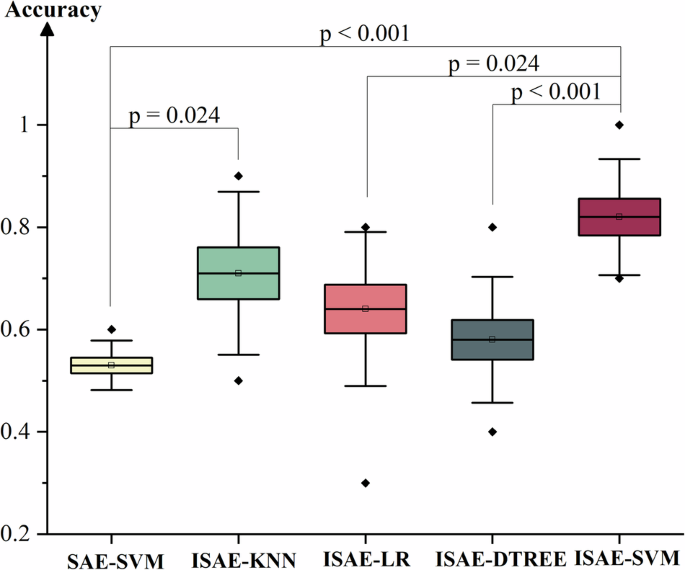
The classification accuracies of five different models were evaluated: SAE-SVM, ISAE-KNN, ISAE-LR, ISAE-DTREE, ISAE-SVM. A two-tailed independent-sample T-test was used to obtain the p-value. Multiple comparisons were corrected using the Bonferroni method (p < 0.05/N, N is the count of items). Solid diamonds represent outliers. The hollow squares represent the mean value. This box diagram is presented as mean/SE/SD. SAE (stack autoencoder), ISAE (improved stack autoencoder), SVM (support vector machine, with parameters C = 3.3 and gamma=0.0005), KNN (K-nearest neighbor with K = 10), LR (logistic regression), and DTREE (decision tree).

Full size image

Distribution of most discriminating functional connections

In this section, we analyze the distribution of the 213 most discriminative functional connections identified through permutation testing. Figure 3 visually illustrates these key connections, emphasizing a reduction in functional connection strength in patients with schizophrenia. To quantitatively assess the distribution of these connections, the brain was divided into six regions: the frontal lobe, occipital lobe, parietal lobe, subcortical system, temporal lobe, and cerebellum. We then analyzed the distribution of the 213 connections both within and between these regions, focusing on both connection strength and quantity. As shown in Supplementary Table 2, for intra-lobar connections, the strengths of connections within the temporal and occipital lobes were greater than those observed in other regions in both groups. For inter-lobar connections, the connection strengths between the frontal and temporal lobes, as well as between the occipital and temporal lobes, were higher than those between other regions in both groups. Supplementary Table 3 shows that, for intra-lobar connections, the quantities of connections within the temporal and occipital lobes were higher than in other regions in both groups. In terms of inter-lobar connections, the quantities of connections between the frontal and temporal lobes, as well as between the occipital and temporal lobes, were greater than those between other regions in both groups. These findings suggest that the frontal lobe, temporal lobe, and occipital lobe are key regions in schizophrenia and may serve as important regions of interest (ROIs) in further research.

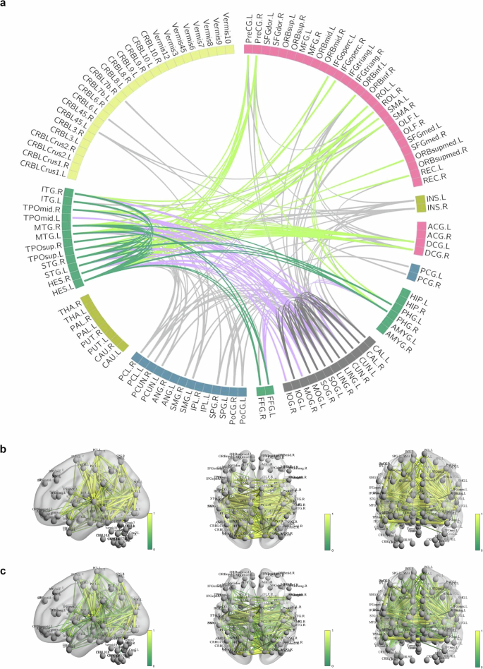
a The Circos diagram representing the distribution of the 213 most discriminative functional connections. b Diagram showing the 213 most discriminative functional connections in the healthy control group. c Diagram illustrating the 213 most discriminative functional connections in the schizophrenia patient group.

Full size image

The results of correlation analysis

We aimed to assess whether discriminating functional connections spanning cognitive function brain area and sensory functional brain area are linked to PANSS scale scores in schizophrenia patients. Pearson correlation analysis was performed on these functional connection strengths and PANSS scale scores, and Fig. 4a–e was drawn accordingly. As shown in Fig. 4a–e, there are a total of five top-down functional connections related to the PANSS scale sub-item scores, including: ORBinf.L to HES.L, ORBinf.L to CUN.R, ORBinf.L to DCG.R, ORBmid.L to HES.L, REC.L to DCG.R. The connection strengths between ORBinf.L to HES.L is correlated with G1 score (p = 0.004, r = -0.403). The connection strengths between ORBinf.L and CUN.R are correlated with P3/G11 scores (p = 0.03 r = −0.33 ; p = 0.022, r = −0.35; respectively). The connection strengths between ORBinf.L and DCG.R are correlated with the N6 score (p = 0.004, r = −0.406). The connection strengths between ORBmid.L and HES.L are correlated with the P6 score (p = 0.046, r = 0.318). The connection strengths between REC.L and DCG.R is correlated with the P7 score (p = 0.015, r = 0.015). Figure 4f is summarized from Fig. 4a–e. As mentioned in the introduction section, ORBinf.L ORBmid.L and REC.L belong to prefrontal cortex (PFC), which is the core of the brain for higher cognitive functions, so we call it as top region. HES.L belongs to temporal lobe, which is responsible for auditory information processing. CUN.R belongs to occipital lobe, which is responsible for visual information processing. The Cingulum bundle (including DCG.R) is a prominent white matter tract that interconnects frontal, parietal, and medial temporal sites, while also linking subcortical nuclei to the cingulate gyrus, which is related with executive control, emotion and so on⁵². So, we call HES.L CUN.R and DCG.R as down region. According to Fig. 4f, we know that five top-down resting functional connections are associated with several positive symptoms, negative symptoms, or general symptoms scores in PANSS scale.

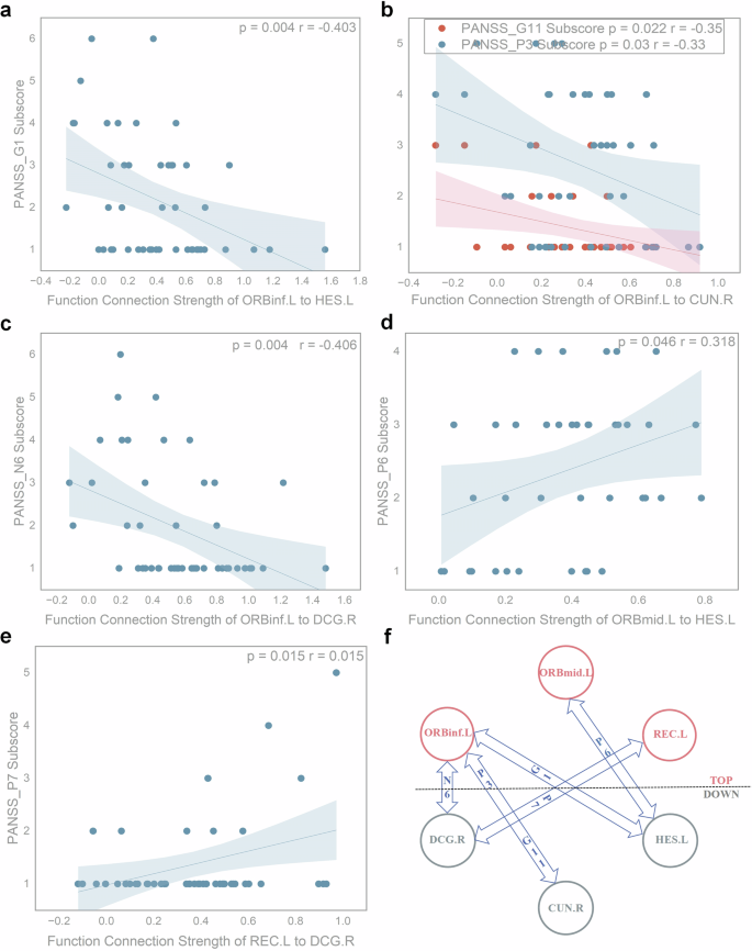
a Pearson correlation result between the connection strengths of ORBinf.L and HES.L and the G1 score (p = 0.004, r = −0.403). b.Pearson correlation results between the connection strengths of ORBinf.L and CUN.R and the P3/G11 score (p = 0.03 r = −0.33; p = 0.022, r = −0.35; respectively). c Pearson correlation result between the connection strengths of ORBinf.L and DCG.R and the N6 score (p = 0.004, r = −0.406). d Pearson correlation result between the connection strengths of ORBmid.L and HES.L and the P6 score (p = 0.046, r = 0.318). e Pearson correlation results between the connection strengths of REC.L and DCG.R and the P7 score (p = 0.015, r = 0.015). f Results of Pearson correlation analysis between top-down functional connection strengths and PANSS scores, based on summaries (a–e). Nodes 1 to 3 represent top regions responsible for higher-order cognitive function, while nodes 4–6 represent down regions responsible for low-level perceptual tasks. PANSS_P3: Hallucinatory behavior; PANSS_P6: Suspiciousness or persecution; PANSS_P7: Hostility; PANSS_N6: Lack of spontaneity and flow of conversation; PANSS_G1: Somatic concern; PANSS_G11: Poor attention. In addition, multiple comparisons were corrected using the Bonferroni method (p < 0.05/N, N is the count of items).

Full size image

The results of spectral dynamic causal modeling (sDCM) analysis

As Fig. 5c shows, compared to healthy controls, top-down effective connections are weaker in patients with schizophrenia, for example, effective connection from ORBinf.L to CUN.R, effective connection from ORBinf.L to DCG.R, effective connection from ORBmid.L to HES.L and effective connection from REC.L to HES.L. At the same time, bottom-up effective connections are stronger in patients with schizophrenia, for example, effective connection from CUN.R to ORBinf.L, effective connection from CUN.R to ORBmid.L, effective connection from CUN.R to REC.L, effective connection from HES.L to ORBinf.L, effective connection from HES.L to ORBmid.L, effective connection from HES.L to REC.L, effective connection from DCG.R to REC.L. Above between-group differences are survived a non-zero criterion with a posterior confidence of 95%.

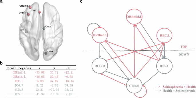
a Brain regions involved in sDCM analysis. b The corresponding MNI coordinates of brain regions in millimeters used for the sDCM analysis. c.The effective connection network, where all lines (connections) form the winning model (connections with a posterior probability > 0.95). The red line indicates that the schizophrenia group has significantly higher connection strength than the healthy group, while the gray line indicates that the healthy group has significantly higher connection strength than the schizophrenia group (probability > 0.95).

Full size image

In this study, we have developed ISAE-SVM model to classify patients with schizophrenia from healthy controls based on COBRE datasets, which include 120 samples. The classify accuracy of 0.82 ± 0.11 was obtained using ISAE-SVM model, which is significantly higher than the results obtained by SAE-SVM, ISAE-LR, ISAE-DTREE models. At the same time, ISAE-SVM model kept a balance between precision and recall, respectively, suggesting the potential of deep learning in searching biomarkers to achieve clinical diagnosis of schizophrenia. In addition, the ISAE-SVM model demonstrated higher FLOPs and a greater total number of parameters, reflecting superior classification performance at the cost of increased computational and storage demands. Based on this accuracy, we found that five resting functional connections, which link brain regions responsible for higher-order cognitive function and brain regions responsible for low-level perceptual tasks, were correlated with sub-item scores on PANSS scale. Further sDCM analysis indicated that schizophrenia’s pathological mechanism involves abnormal information interaction between the regions responsible for higher cognitive function and the regions responsible for lower perceptual tasks. In schizophrenia, the top-down cognitive control is weakened, and the bottom-up signaling is enhanced.

On one hand, we detected attenuated effective connections from ORBinf.L to CUN.R, from ORBinf.L to DCG.R, from ORBmid.L to HES.L, and from REC.L to HES.L in patients with schizophrenia. These findings suggest a weaker top-down cognitive control in patients with schizophrenia compared to healthy controls. Our findings are consistent with previous studies that weakened top-down control causes cognitive impairment in schizophrenia. For instance, regarding suspiciousness or persecution delusions, a positive symptom of schizophrenia, studies have demonstrated that top-down influences (specifically signals along the pathway from the inferior frontal gyrus (including ORBinf) to the lateral occipital cortex (including CUN)) are constrained in schizophrenia⁵³. This suppression may contribute to the development of suspicious or persecution delusions^52,54. Moreover, the weakened top-down control in schizophrenia is likely associated with reduced activation in the prefrontal cortex (PFC), including regions such as ORBinf.L, ORBmid.L, and REC.L, impairing the PFC’s ability to suppress irrelevant sensory information^55,56. Additionally, insufficient top-down predictions may fail to adequately guide sensory processing, leading to misinterpretation of sensory inputs, which is also implicated in suspiciousness or persecution delusions⁵⁷. With respect to the negative symptom of lack of spontaneity and flow of conversation, healthy adults rely on top-down pathways to generate predictive information, thereby attenuating neural responses to expected stimuli. In contrast, patients with schizophrenia exhibit diminished top-down predictive signals, resulting in heightened activity in primary sensory cortices⁵⁸. Furthermore, this weakened predictive processing has been linked to reduced gray matter volume in the superior temporal gyrus⁵⁹. For poor attention, another core symptom of schizophrenia, numerous studies have reported impaired top-down attentional modulation of non-social stimuli. For example, compared with healthy controls, patients with schizophrenia show abnormal prefrontal activations during oddball tasks⁶⁰ and fail to suppress activity in limbic regions, including the amygdaloid nucleus⁶¹.

On the other hand, we detected enhanced effective connections from CUN.R to ORBinf.L, from CUN.R to ORBmid.L, from CUN.R to REC.L, from HES.L to ORBinf.L, from HES.L to ORBmid.L, from HES.L to REC.L, from DCG.R to REC.L. These findings suggest that stronger bottom-up signaling transmission causes perception dysfunction in schizophrenia. Consistent with this, previous studies have demonstrated that patients with schizophrenia exhibit hyperactivity in early sensory regions, such as the auditory and visual cortices, even in the absence of corresponding external stimuli⁶². Furthermore, the aberrant salience hypothesis posits that hallucinations (a classic perceptual disturbance) arise from the direct experience of aberrant salience attributed to internal representations¹⁶. This framework provides a potential explanation for hallucinations, suggesting that the brain’s overrepresentation of sensory input may lead to false perceptions. Coincidentally, studies from several laboratories also have found that perceptual processing measures are consistent with bottom-up theoretical formulations^62,63,64. That means the presence of abnormalities in bottom-up processing may be the cause of impairment in the perception (eg. hallucination) of patients with schizophrenia^65,66. There’s another explanation that diminished P50 suppression, a neurophysiological indicator of sensory gating that pertains to the capacity of the brain to disregard superfluous sensory stimuli, is commonly detected in patients with schizophrenia, thereby suggesting an augmented bottom-up sensory transmission¹⁶. These stronger bottom-up signaling, when combined with overreliance on perceptual priors, could possibly cause disturbance of perception (eg.hallucinations)⁶⁷.

A major conclusion of this study is that weaker top-down cognitive control and stronger bottom-up signaling together constitute the pathogenic mechanism of schizophrenia, which just verifies our hypothesis. As discussed earlier, weaker top-down cognitive control might bring about the cognitive impairment symptoms of schizophrenia, while stronger bottom-up signaling could potentially cause the perceptual damage symptoms of schizophrenia. However, schizophrenia is a comprehensive and heterogeneous disease, and its most striking symptoms include both cognitive impairment and perceptual damage, so the weakening of top-down cognitive control and the enhancement of bottom-up signaling can be its fundamental pathogenic mechanism. Our findings are consistent with the three-component model of mental illness proposed by Emrich et al. ⁵⁶. According to this theory, mental illness is principally made up of three components: firstly, sensory input (“sensualistic” component, bottom-up process); secondly, the internal production of concepts (“constructivist” component, top-down process); and thirdly, control (“censor” component). The third component is identified as the interaction between the other two components and it is not attributed to a specific spatial area in the brain. As a major mental illness, schizophrenia is also caused by the abnormal interaction of top-down components and bottom-up components, which may be one of the reasons why the disease has multiple heterogeneous symptoms.

Another significant contribution of this study is the development of a promising intelligent diagnostic tool for schizophrenia: the ISAE-SVM model. With recent advancements in artificial intelligence, the ability to characterize and classify schizophrenia has improved considerably. Among these techniques, autoencoders and support vector machines (SVMs) have been extensively explored due to their capability to handle high-dimensional and complex datasets. Previous studies have demonstrated that, regardless of the input feature type, autoencoders can effectively capture latent feature patterns in high-dimensional neuroimaging data through nonlinear transformations and dimensionality reduction^23,24. For instance, Gang Li et al. developed a deep canonically correlated sparse autoencoder (1D model), achieving 80.53% classification accuracy when using single nucleotide polymorphisms (SNPs) and fMRI voxel values as features⁶⁸. Afshin Shoeibi et al. utilized a convolutional autoencoder (2D model) to extract features from rs-fMRI functional connection matrices, achieving 72.71% classification accuracy when combined with a wolf optimization-based interval type-2 fuzzy regression algorithm⁶⁹. Huaiqiang Sun et al. developed a 3D convolutional autoencoder to learn morphological patterns from T1-weighted structural MRI, where classifiers trained on autoencoder-derived features outperformed those trained on conventional morphological features by 10 percentage points, achieving 73.44% and 71.85% classification accuracy on internal and external validation datasets, respectively⁷⁰. Meanwhile, SVMs have demonstrated robust classification performance by locating the optimal decision hyperplane in the high-dimensional feature space constructed from latent representations²⁵. Previous studies have shown that SVM-based models achieve classification accuracies ranging from 70.23% to 81.28% when using various features, including static and dynamic rs-fMRI indexs⁷¹, group-difference functional connections selected via T-test, Kendall Tau, and Fisher’s score⁷², voxel-wise density values of white and gray matter⁷³, subnetwork-level functional connections⁷⁴, and anticorrelated network’s functional connections⁷⁵. However, these models often suffer from the vanishing gradient problem during training, which can impede their learning efficiency^27,28. Additionally, noise and artifacts in signals further degrade their capacity to extract robust features and generalize effectively^29,30. To address the aforementioned issues, this study integrates the strengths of autoencoders and SVMs to develop the ISAE-SVM model, which introduces several improvements to the traditional stacked autoencoder (SAE) framework. Specifically, Dropout layers are incorporated to prevent overfitting, while short connections are introduced to mitigate gradient vanishing during training. Additionally, the cost function is optimized by fully leveraging sample information, thereby enhancing the model’s learning capability. The high-dimensional latent features transformed by the ISAE network are subsequently fed into an SVM classifier for binary classification. Notably, since the input and output dimensions of ISAE remain the same, its primary function is to transform input features into a new coordinate system, facilitating the SVM’s ability to define an optimal decision boundary in the high-dimensional latent space. Experimental results demonstrate that the proposed ISAE-SVM model achieves an average classification accuracy of 82%, surpassing many existing approaches. Our findings underscore the potential of AI models as auxiliary tools for the clinical diagnosis of schizophrenia.

The main strength of this study is that it elucidates the abnormal dynamic causal interaction between brain regions responsible for higher cognitive functions and multimodal brain regions involved in lower perceptual tasks in patients with schizophrenia. At the same time, this study proposed a potential clinical diagnostic tool for schizophrenia. The current study has several limitations. On one hand, personalized clinical data, such as details on drug therapy, were not included in the analysis. Future research should incorporate more specific clinical information to enhance the understanding of schizophrenia’s pathogenesis. On another hand, there is a need to integrate multi-modal imaging data to identify comprehensive biomarkers that can support the clinical diagnosis of schizophrenia.

In conclusion, our research indicates that schizophrenia may originate from diminished top-down cognitive control and enhanced bottom-up signal transmission. The abnormal dynamic causal interactions between brain regions that process multimodal sensory information and those implicated in higher-order cognitive functions could potentially elucidate the intricate and diverse clinical manifestations observed in schizophrenia. This integrated analysis of the interaction between top-down and bottom-up pathways offers a new research method to investigate schizophrenia. In addition, the ISAE-SVM model based on deep learning proposed in this study achieved good classification accuracy, which is conducive to assisting the clinical diagnosis of schizophrenia. Furthermore, our research underscores the importance of the prefrontal cortex (including ORBinf.L, ORBmid.L, and REC.L), which is the core brain region responsible for high-order cognitive functions and complex social behaviors⁵⁴. It also highlights the role of three multimodal lower perceptual brain regions (including HES.L, CUN.R, and DCG.R), which are responsible for the initial processing of auditory information, the early processing of visual information, emotional regulation, and social function in the context of schizophrenia, respectively^{76,77,78,79,80,81,82}.