Weather sensing with structured light

Introduction
The interaction of optical fields with disordered and complex media has been an area of considerable interest for many researchers1,2,3,4,5,6,7. Such media commonly induces intensity and phase distortions that can be disruptive for optical communications and imaging systems8,9,10,11,12,13,14,15. However, these optical distortions are directly dependent on the environment that the complex media is situated within and therefore measuring these distortions could be used as a accurate way to sense changes in the world around us1,10,12,16. Free-space optical applications, such as space division multiplexing, quantum key distribution, optical imaging, and optical sensor systems are all acutely affected by the atmosphere17. The core challenge faced during propagation through the atmosphere is that these optical beams experience path dependent optical distortions that are accrued over hundreds or thousands of meters of propagation18. Along this path, there are time-dependent and random variations in the temperature of the air and wind speed resulting in density changes19. These subsequently result in spatial and temporal changes in the refractive index structure of the propagation channel that lead to complex optical aberrations that can disrupt imaging, sensing, and communication systems15,20,21. One burgeoning area of research is the mitigation of the crosstalk from the aberrations that arise in free space optical (FSO) channels to enable space division multiplexing (SDM), where turbulence leads to crosstalk between independent data channels and can dramatically limit the performance of communication systems22. It is common to describe each channel in an optical SDM system as a set of orthogonal spatial modes such as Laguerre-Gaussian or Hermite Gaussian modes. Laguerre-Gaussian (LG) modes are naturally eigenmodes of circular apertures, where these modes are characterized by orthogonal mode indices ℓ and p, corresponding to the azimuthal and radial components, respectively23. These beams have a transverse complex amplitude profile of (Aleft(rright)exp left(iell phi right)) and carry an Orbital Angular Momentum (OAM) of ℓℏ per photon with r and ϕ as the radial and angular coordinates, respectively24. Optical aberrations or misalignment between the propagation axis of the optical field and the axis of the receiver have been shown to have distinctive crosstalk between received modes that has been referred to as OAM spectroscopy11,25,26. These spectra have previously been used to realize digital spiral imaging for determining changes of phase and amplitude of an optical beam27,28,29. More generally, OAM spectroscopy can be used as a tool to probe any geometrical and structural properties of matter that impact the propagating of OAM beams28. During propagation in long-distance turbulent channels, each LG mode experiences unique optical distortions10,30. These OAM-dependent distinctive interactions could be leveraged to extract the environmental origins of the observed inter-channel crosstalk and used to create enhanced hybrid communication and environmental sensing systems.
Turbulence in the atmosphere can be generated by the mixing of air with different temperatures, where this mixing forms eddies as the energy is dissipated. These eddies have a spiral structure, similar to that of hurricanes, where their size, distribution, and movement are a direct result of weather parameters like temperature distributions and wind speed31. Various technologies can be deployed at fixed points to test wind-speed, such as sonic or mechanical anemometers32,33. Similarly for temperature thermistor or thermocouples can be placed at specific physical locations to monitor turbulence conditions34,35,36. The commonly observed optical aberrations in free-space are a direct result of propagation through many eddies over a turbulent channel, where these aberrations can be linked to changes in weather. Each interaction will result in local changes in the propagation direction and phase, which after propagation will lead to spatial changes in intensity that evolve during propagation as interference occurs between the locally tilted wavefronts. This effect is the key contributor to scintillation of the optical signal. Experimental techniques such as scintillometry track the time varying intensity changes and computationally compare them to estimated channel models to infer environmental parameters37. Typically, commercial scintillometers measure the refractive index structure parameter, ({C}_{{{rm{n}}}}^{2}), which can give an estimate of heat variation across an operational range that can span from hundreds of meters to several kilometers37,38. These measurement approaches typically require long integration times (tens of minutes to over one hour) to achieve acceptable accuracies for particular applications.
Solely measuring global changes in intensity does not allow for direct determination of the key parameters such as inner scale value, l0, which are closely related to the structure of the eddies in turbulence. Multi-aperture scintillometers (MASS), where multiple apertures simultaneously record the intensity variations38,39, have been suggested to improve the resolvability of l0 and ({C}_{{{rm{n}}}}^{2}). Recently, wavefront sensors combined with machine learning have been demonstrated to offer further improvement by substantially increasing the number of effective apertures40. However, the natural evolution of eddies has a rotational spatial structure, therefore measurements of the spiral motion will be projected into a pixelated coordinate system. Conversely, as shown in Fig. 1, OAM beams twist as they propagate creating an optical vortex along their axis of propagation, which is structurally similar to atmospheric eddies created by turbulence. This suggests measurements of OAM content from light interaction with atmospheric eddies could provide improved determination of key parameters about a particular physical channel.

a Turbulent eddies are induced in due to the time varying changes in temperature and pressure along an free-space channel, represented by a computation fluid dynamic simulation of hot (red) and cold (blue air mixing in a particular volume. b Optical beams that carry Orbital Angular Momentum (OAM) are distorted over the full length of the channel, resulting effects such as vortex splitting, where high order vortices, such as ℓ = 3 breakup in to multiple, spatially displaced ℓ = 1 vortices. Beam propagation depicted in separately from turbulent volume to clearly see the deformation over propagation through volumetric turbulence. c This result in unique OAM power spectra that can be used for measuring changes in the environment.
This article demonstrates experimentally that the use of an optical probe carrying OAM and an OAM sensitive receiver can be used as a tool to measure both the wind speed and temperature in an electronically controlled 36 m turbulent FSO channel. A measurement resolution of 0.49 °C and wind speed variations of 0.029 ms−1 were achieved via the use of a Support Vector Machine (SVM) regression algorithm, trained on the inter-channel crosstalk between OAM modes measured by a passive mode-sorter, using an ℓ = 3 optical probe beam. The OAM mode-sorting can be considered as a form of all-optical pre-processing to support feature discovery and experimentally revealed features that were embedded in the OAM spectra that could be used reliably with machine learning regression models. The recorded crosstalk gives a measurement of the power distribution of OAM within an optical beam concerning a specific measurement axis. Changes in the total OAM or movement in the position of an optical vortex will lead to distinctive power distributions, also referred to as OAM spectrum, that can be used for monitoring the structure of turbulent fields. When a Gaussian mode that has OAM of ℓ = 0 propagates through the turbulence-induced atmospheric eddies, randomly distributed pairs of phase vortices are created with ℓ = −1 and ℓ = 1. Where this effect is common place in any optical system where speckle aberrations are observed due to the interference of multiple deflected optical wavefronts41. As pairs are produced, the total OAM of ℓ = 0 is maintained due to the conservation of angular momentum10,30,42. However, the center of each vortex will not align with the measurement axis and therefore will result in the distribution of OAM with a mean not equal to the ℓ of the input beam and with a width determined by the number and distribution of vortices. As the channel distorts this beam, the variation in the mean OAM will be directly related to the interactions of turbulence and the light mode10,30. Therefore, measurement parameters such as average OAM and OAM distribution are closely related to the environmental conditions of the channel.
We expect this technique could be used as an effective path-integrated and potentially channel-resolved weather monitor. This approach could also be used as a weather monitor to increase the resolution of weather prediction systems43,44,45. There is a key challenge in predicting extreme weather events, partly due to the limited sampling generally available for weather mapping from highly localized weather stations46. Path-integrated weather monitors could provide unique data for future weather models as this approach can provide an increased accuracy over scintillation index based measurements of wind speed and temperature by a average gain factor of 4.5 and 3.54, respectively, are specifically calculated in Discussion section. Our presented approach suggests a significant improvement over widely used scintillometers for environmental monitoring, such as tracking heat fluxes in the Amazonian rain forest47. The system architecture is also ideal for hybrid FSO communications and environmental sensing, as the de-multiplexer could simultaneously be used for SDM channel demultiplexing and channel monitoring. Such hybrid approaches could be leveraged by network control and management tools to enhance the resiliency of optical networks by adapting to changes in weather conditions.
Results
Atmospheric Turbulence
Atmospheric turbulence is governed by the fluid dynamics of a particular channel and has a key parameter called Reynolds number, ({{rm{Re}}}). This number is a numerical relationship between viscous and inertial force where low ({{rm{Re}}}) signifies the dominance of viscous forces leading to constant flow and high ({{rm{Re}}}) signifies inertial forces dominance leading to more chaotic behavior. This can be expressed as ({{rm{Re}}}=frac{VL}{nu }), where ν is the kinematic viscosity, V is the velocity of flow, and L is the characteristic linear dimension of the fluid, respectively48. Fluid flows can be categorized into two main types: laminar and turbulent flows. Laminar flow is a smooth, orderly fluid movement with parallel layers and minimal mixing, typical of slow-moving, viscous fluids. In turbulent flow, the velocity and direction of flow at a specific point undergo continuous and random changes, resulting in eddies and rapid fluctuations in flow characteristics. In 1922, Lewis Fry Richardson developed one such early model known as the energy cascade theory, which explains turbulence as a cascade of random turbulent eddies with various scale sizes, that range from the smallest eddy known as the inner scale, l0 to the outer scale, L0, that defines the largest thermally stable volume of air48. Large areas of air are heated, by the sun for example, forming large scale turbulent eddies, L0, which subsequently break down further into smaller eddies under the influence of inertial forces until the eddy reaches the inner scale when the energy within that eddy dissipates into heat. For the majority of naturally occurring turbulent environments, we only consider the propagation of optical beams through a restricted range of Reynolds numbers linked to the ratio of inner scale to outer scale by the relationship,
The critical parameter that affects optical fields is the refractive index fluctuation that results from the eddies formed48. The turbulence power spectrum models can give the statistical averages of the random variation process of the atmosphere. The turbulence mixes different layers of air forming eddies and as pressure is locally constant, this results in a spatial variation of density, ρ, that leads to spatial variation in refractive index, n. The average size of the smallest turbulent eddies is given by,
where ν is the kinematic viscosity and ϵ is the energy dissipation rate of atmosphere. Kinematic viscosity ν is a function of temperature and ϵ is related to both temperature and wind speed distribution49. The refractive-index structure constant ({C}_{{{rm{n}}}}^{2}) which is a measure of the local turbulence strength can be deduced from the temperature structure constant ({C}_{T}^{2}) by
where P is pressure, T is temperature. The phase distortion can be described by a coherence length scale of the turbulence known as the Fried parameter r0.
Here, k is the wave number, and ζ is the zenith angle1. Through the above equations and analysis, it is expected that both temperature and wind speed have a joint effect on the turbulence parameters r0 and l0.
Turbulent flow is a nonlinear and multiscale process governed by the Navier-Stokes equations. As direct solving of Navier-Stokes equations is computationally challenging, statistical models are commonly used to represent the interactions in atmospheric channels instead of purely computational approaches. One widely used model is the Large Eddy Simulation (LES), which aims to reduce computational costs by filtering out the smallest length scales, which are computationally intensive, through low-pass filtering of the Navier-Stokes equations, effectively eliminating fine scale information50. Using computational fluid dynamics (CFD) modeling software (OpenFOAM v2212), we implemented an LES to create a turbulence channel numerically that could provide an estimate of the spatial and temporal variation of key turbulence parameters. This was subsequently used to optimize the design of an experimental turbulence simulator. Turbulence is commonly produced in a laboratory setting by mechanically forcing the mixing between warm and cooled air in a central mixing area51. To replicate this, we simulated a system that includes heat reservoirs for both warm air and cool air that will be mixed in a central chamber. The CFD mesh was created to represent a physical environmental emulator that is 2 m in length, 0.15 m in height, and 0.2 m wide with 15 air inlets from each heat reservoir. To relate the fluid dynamic properties of the channel to turbulence parameters l0 and r0, in the CFD simulation spatial field distribution of Tcfd, Pcfd, and ({vec{V}}_{{{rm{cfd}}}}) was recorded every millisecond for the mixing chamber and processed using equation (2) and (4) for l0 and r0, respectively. To investigate a range of different environmental conditions the speed of the air from the reservoir to the mixing chamber, V, was varied, along with different temperature differences across the chamber. V ranged from 3 ms−1 to 11 ms−1 in intervals of 2 ms−1, and the temperature difference between the hot air and cool air Δ T = Thot − Tcool spanned from 5 °C to 25 °C in intervals of 5 °C, with Tcool fixed at 21 °C. The calculated l0 and r0 are shown in Fig. 2, where a distinctive relationship between these values and temperature and flow rate is observed.

a The Fried parameters under 25 different temperature and wind speed combinations. b The inner scale under the same 25 different temperature and wind speed combinations.
Structured Light Interaction with Environment
LG modes form a complete basis set of orthogonal modes, meaning that any complex amplitude profile can be represented as a weighted superposition of these spatial modes, i.e., a spatial modal spectrum. A notable behavior observed for OAM modes that are aberrated is called vortex splitting, where a beam that carries an OAM ℓ = m, will break up into m vortexes of ℓ = 1 that are spatially separated. While the total orbital momentum is conserved, it is not entirely localized at the original beam propagation axis. The average displacement of the vortices from the axis center is directly related to the D/r0 of the atmospheric channel30. To obtain the expected OAM spectrum after propagation through a bulk turbulent channel with different combinations of r0 and l0, we performed a propagation simulation based on the split-step algorithm using 120 segments to simulate a representative turbulence channel of 1200 m. Each screen was calculated using the von Kármán spectrum and underwent sub-harmonic correction30,52.
To investigate the specific connection between the OAM spectrum and the simulated turbulent channel, 10 Fried parameters, r0, and 10 inner scales, l0, were tested, where each combination was simulated to provide 100 effective channel conditions. For each combination, 100 realizations were computed to account for the random variation in the channel. The selected spectra for a beam with ℓ = 3 and p = 0 are shown in Fig. 3a. We can see that the height and shape of the curve change with the turbulence parameters. The spectra features were subsequently analyzed by considering a weighted sum of the spectral components,
and the variance in the spectra,
where Aℓ is the normalized amplitude of each OAM mode with a spiral phase index of ℓ, (mu =frac{1}{N}{sum }_{{ell }_{min }}^{{ell }_{max }}{A}_{ell }^{2}) and N is the total number of OAM modes. Changes in r0 and l0 were shown to lead to continuous variation in both η and σ2, as shown in Fig. 3b, c. In real air turbulence channels, r0 and l0 are functions of T and V. Therefore, we propose that each can be defined as a function η = f(r0, l0) = g(T, V) and ({sigma }^{2}={f}^{{prime} }({r}_{{{rm{0}}}},{l}_{{{rm{0}}}})={g}^{{prime} }(T,V)). Explicit derivation of these functions is challenging due to the statistical approaches to representing real-world turbulence accurately. However, regression analysis of real-world turbulence can yield a model that strongly suggests a direct link between the OAM spectrum and changes in T and V.
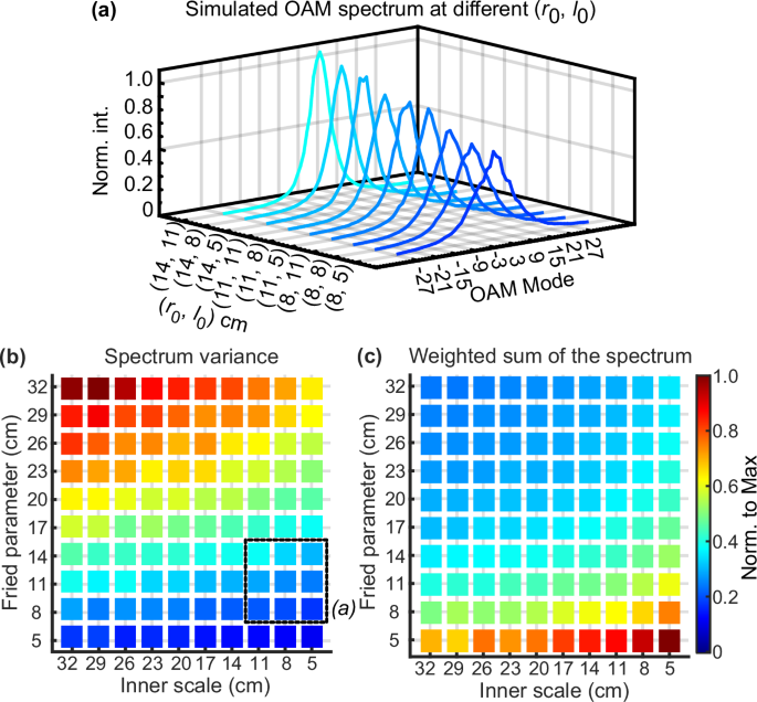
a OAM spectra for a range of l0 and r0 values when an OAM beam with ℓ = 3 is propagated over a simulated optical channel. b The spectrum variance, σ2, is calculated for 100 different turbulence channels with split-step propagation simulation. Dashed box indicates the spectral plots associated with these data points in (a). c The weighted sum of the spectral components η, calculated for 100 different turbulence channels with split-step propagation simulation.
Environmental Emulator
Key to the development of any reliable sensor technology is the availability of appropriate controllable test facilities to generate known environmental conditions. Based on the numerical simulations, an experimental environmental emulator was developed to emulate the multiple interactions with turbulence expected in long distance optical propagation. Our constructed turbulence emulation chamber had computer controlled temperature and wind speed, and is shown in Fig. 4. Warm air was heated using electrical heaters, embedded in the thermal mass of igneous rock, and the temperature of the air could be varied up to approximately 15 °C above ambient room temperature. Digital thermometers were utilized to establish a feedback loop to stabilize the heating of the warm air chamber at the target temperature. As mixing of hot and cold air was required, cooler air of approximately 21 °C was mechanically mixed with hot air by 30 fans evenly spaced over the 2 m length of the chamber. The wind speed produced by fans could be precisely adjusted from 0 to 4.95 ms−1, using the calibrated lookup tables relating wind speed to the rotational frequency of the fans. The latter was controlled independently for each fan using a custom closed-loop driver board employing dedicated multi-channel fan controller ICs (Maxim Integrated MAX31790), interfaced to the LabVIEW-based experiment control software over a serial USB connection.
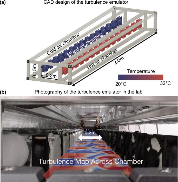
a The Computer Aided Drawing (CAD) design of the emulator, with cold, hot, and mixed air chambers. The dimensions of mixed air chamber are 0.15 m, 0.2 m, and 2 m in height, width, and length, respectively. b A photograph of the emulator is superimposed with the temperature distribution figure obtained from Computational Fluid Dynamics.
Experimental Measurements
While continually monitoring temperature and wind speed, the temperature difference, ΔT, and average wind speed were varied over the range of 0.9 °C to 13.8 °C and 0.68 ms−1 to 1.37 ms−1, respectively. ΔT was achieve through heating air above the ambient room temperature of 21 ± 1 °C. For each condition, OAM optical beams with ℓ values between ℓ = −3 and ℓ = 3 were transmitted over the turbulent channel. We time-averaged 3 s of recorded spectra to reduce the effects of random spectral features that arise from complex turbulence processes10. To prevent saturation from long exposures, the OAM spectrum was measured at a frame rate of 30 Hz with a 30 ms exposure time, providing a time-averaged result as turbulence fluctuated at the Greenwood frequency (GF) for a given environmental condition. All recorded images over the 3 s measurement window were summed, and the time-averaged results were computed (see Methods Section). The GF of the channel varied with changes in wind speed and turbulence strength, as measured across all our measurement points (see Methods Section). The maximum measured frequency was approximately 388 Hz, corresponding to a coherence time of 2.58 ms. All data was labeled with time stamps, real-time temperatures, and wind speed to allow for accurate data analysis and machine learning training. The variation of the OAM spectra was observed to show a distinctive pattern that follows the temperature changes, Fig. 5a, and changes in wind-speed, Fig. 5b The obvious similarity between the adjacent curves in Fig. 5b, c indicates that the OAM spectrum is not entirely random. The variation in spectrum variance and weighted sum for temperature difference and wind speed is similar, but not identical, to the variation in the Fried parameter, r0, and inner scale, l0, of a simulated turbulent channel using CFD, as shown in Fig. 3. This is expected due to the coupled nature of r0 and l0 in relation to changes in temperature and wind speed, as outlined in Section 2. These similar features serve as the basis for training our SVM model. We note that the variation in trend seen in Fig. 5e at low windspeed, compared to Fig. 3c, may result from small changes in the fluid dynamics of the experimental chamber compared to the idealized simulation. These changes include variations in air exhaust rate, static pressure on individual fans, and local airflow rates. Such effects would be minimized in a real-world deployment of this measurement approach. We note that this does not substantially affect our accuracy in recovering environmental parameters based on experimentally trained regression models.
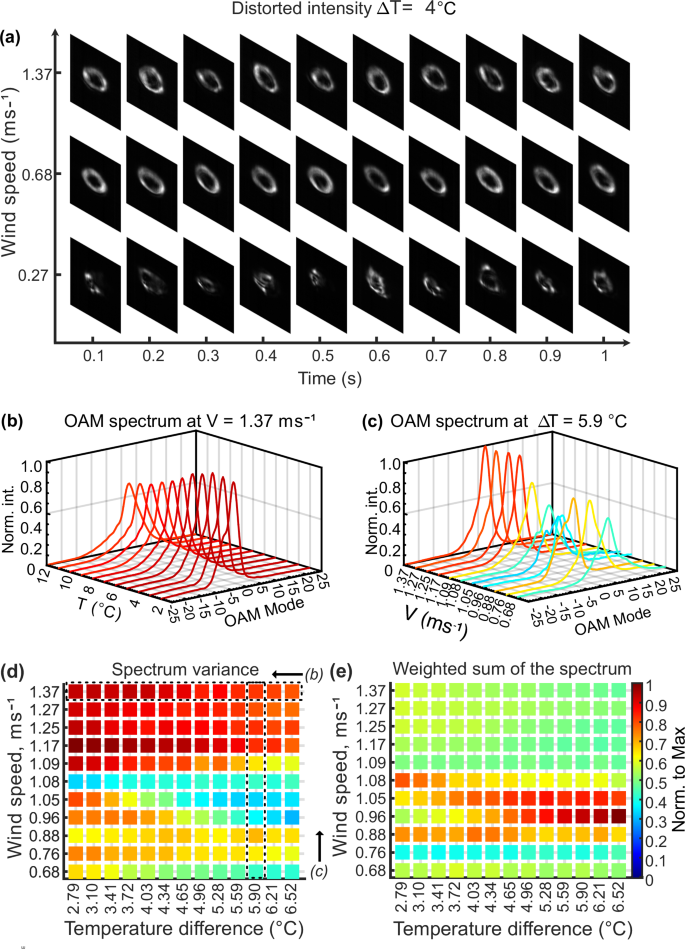
a The received OAM beams are distorted by changes in wind speed and temperature, with these distortions varying over time. As a result, any single image is not fully representative of the channel’s spatial variance. Therefore, time-averaged OAM spectra are measured to capture the statistical variation in aberrations over the 3 s measurement window. b OAM spectrum curves for a wind speed of V = 1.37 ms−1 with ΔT varying from 2 to 12 °C. c OAM spectrum curves for ΔT = 10 °C with wind speeds varying from 0.68 to 1.37 ms−1. d The experimental spectrum variance, σ2, where boxes indicates the spectral plots associated with these data points in (b) and (c). e The weighted sum of the experimental spectral components, η.
To analyze the spectra, we can compute two metrics for the experimental observations, η, equation (5), and σ2, equation (6). Both metrics have distinctive structures, suggesting an underlying function determining the observed result. It is proposed that the intersection between these underlying functions can be used to simultaneously measure the wind-speed and temperature of our turbulent channel simulator. However, due to the coupled nature of the system, machine learning tools can be readily used to determine a hyperplane defined by input features. Therefore, an SVM algorithm is used to perform regression analysis. In this algorithm, the kernel function is a critical component that determines the shape and dimensionality of the decision boundary. We chose a polynomial kernel to map the data into a higher-dimensional space using a polynomial function.
where, α, β, and γ are kernel parameters that influence how the data is transformed into a higher-dimensional space. Xi and Xj represent the feature vectors. The parameter α governs the impact of individual training samples on the decision boundary. Higher values of α result in more elaborate decision boundaries that closely align with the training data, β introduces an offset to the decision boundary, while γ denotes the polynomial degree within the kernel function, thereby dictating the complexity of the decision boundary.
The OAM spectrum with range ℓ = ±25 was used as the input for SVM training, with data labeled for both wind speed and temperature differences recorded during the experiments. These labels were determined by measuring the average of 10 thermometers spaced evenly over the channel emulator and calibrated tachometers on each fan. The polynomial order of γ = 2 was chosen to prevent overfitting of the data due to random fluctuations arising from the turbulence. Each training data point is the average of 90 spectra, which represents the data collection interval of 3 seconds. Out of 3897 samples collected from various channel scenarios, 90% were randomly chosen for model training using 5-fold cross-validation. All data used for model for verification was recorded separately from the data used for training. Verification dataset covering the temperture range and wind-speed covering the range 1.0 °C to 12.2 °C and 0.68 ms−1 to 1.37 ms−1 respectively, comprising 390 samples (10% of total data collected), was recorded several days after the training data and soley used for the results presented in Fig. 6. This highlights that this approach could be used for real-world applications in future studies. The remaining 10% were used as test data to evaluate the trained model and calculate measurement accuracy. In total, 3 groups of data collected on different days were aggregated to ensure results were not solely related to a specific channel realization. The measurement of wind speed and temperature by the trained SVM model are shown in Fig. 6a, b, respectively. We trained two separate models using the same complete training data to comprising the same wind speed and temperature measurements. and we used the standard deviation of the measurement results to represent the accuracy of the SVMs based measurement approach. As shown in Fig. 6, there is an increase in measurement error. This is due to higher temperatures typically inducing larger variances in turbulence-induced aberrations, where the full spectrum may not be fully captured within a 3 s measurement window. Therefore, increased measurement time or dynamic averaging based on conditions may be required. The highest accuracy achieved for temperature and wind-speed was 0.49 °C and 0.029 ms−1 respectively.
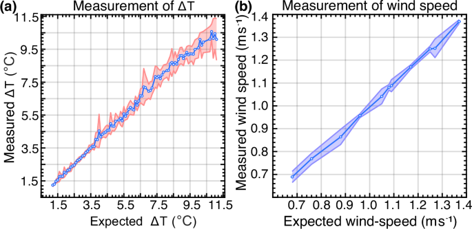
a Measurement of temperature difference ΔT, plotted against the expected ΔT from experimental ground-truth measurements obtained using multiple thermometers placed throughout the system. b Measurement of wind speed, plotted against the expected wind speed from experimental ground-truth measurements using air-flow calibrated fan-speed monitoring. The colored region around the central trend line represents the measured standard deviation at each point with respect to the corresponding expected measurement. All data used for measurements were recorded separately from the data used for SVM training.
Discussion
Our experiments so far have focused on the decomposition of the optical field into its constituent OAM modes. However, other methods for analyzing the received optical intensity can be considered. To determine the benefit of OAM decomposition, training based on the received intensity profile and the scintillation index were considered as well. Using direct imaging onto a CCD camera, the intensity profile was measured simultaneously with the output of the mode sorter to allow for direct comparison with the same environmental conditions, see Methods section. First, the SVM model was trained using two vectors, which were the summation of the pixels along horizontal and vertical axes, respectively, averaged for data recorded over a time window of 3s. In the second case, using the data from the directly imaged optical field, the scintillation index was calculated for each pixel occupied by the beam over a 3 s time window, ensuring that the size of training data was the same as that used for the SVM models based on OAM spectrum and OAM intensity profile measurement. Therefore, in the presented results the scintillation index (SI) for each 302 pixels that the beam covered on the camera was determined and used for model training, see methods section. This is equivalent to dividing the receiver into 302 independent apertures. The direct comparison of measurement accuracy resulting from the OAM-based model as well as the two aforementioned alternative implementations is indicated in Table 1.
To indicate the performance increase achieved for OAM-based measurement approaches, we draw comparison with a reference measurement approach based on SI, as this is similar to multi-aperture scintillometers that are commonly used. Additionally, we draw comparison between two channel OAM-based measurement approaches that leverage OAM Intensity or OAM spectrum measurements. We can consider a range of accuracy gain factors between the measured root-mean-square-error (RMSE) of determined temperature-difference (Δt) and wind-speed (V) compared to the measured ground-truth, shown in Table 1. To first consider the accuracy gain of using OAM spectral compared to SI measurements by computing
to consider improvement in measurement of ΔT, where Nℓ is the number of integer steps in ℓ. As NℓN = 7 the average accuracy gain is ({G}_{Delta {{{rm{T}}}}_{{{rm{SI}}}}}=3.54). The accuracy gain for the measurement of wind-speed
where ({G}_{{{{rm{V}}}}_{{{rm{SI}}}}}=4.5). This indicates that SI is less accurate measure then spatially resolved measurement techniques, such as the OAM spectrum (OAMS) based measurements. Both intensity profile (IP) and OAMS are directly linked to the changes in spatial bandwidth that occur during propagation over the turbulent channel. Therefore, we expect the performance of each approach to be closer matched in accuracy, as shown in Table 1. The accuracy gain of using OAMS compared to IP measurements can be determined by computing
to consider improvement in measurement of ΔT, where the average gain is ({G}_{Delta {{{rm{T}}}}_{{{rm{IP}}}}}=1.14). The accuracy gain for the measurement of wind-speed
where ({G}_{{{{rm{V}}}}_{{{rm{IP}}}}}=1.39). This highlights that OAMS offers the biggest measurement accuracy gain for wind-measurements. These gains are for considering all transmitted modes, including beams that don’t carry any OAM, specfically ℓ = 0. Therefore, we can determine the accuracy gain from using a OAM probe beam with ℓ = ∣3∣ by computing
to consider improvement in measurement of ΔT, where ({G}_{Delta {{{rm{T}}}}_{ell = | 3| }}=1.39). The accuracy gain for the measurement of wind-speed by computing
where ({G}_{{{{rm{V}}}}_{ell = | 3| }}=1.60). These results confirm that OAMS, while utilizing an OAM probe improves the performance of weather sensing compared to alternative approaches. The marked improvement of over 4 times compared to SI, which is a commonly used approach for channel monitoring. Additionally, the usage of OAMS compared to IP, utilizes 21 OAM sampled real-valued intensities as compared to 600 real-valued pixel. The ratio of these two values indicates a reduced the required information by a factor of 28.6. We note there is variability in the accuracy for the SI due specific turbulent conditions. Modes carrying OAM provided an improvement in sensitivity over modes with ℓ = 0. For wind speed, ({G}_{{{{rm{V}}}}_{ell = | 1| }}=1.56) and ({G}_{{{{rm{V}}}}_{ell = | 2| }}=1.38), and similarly for ΔT, where ({G}_{Delta {{{rm{T}}}}_{ell = | 1| }}=1.60) and ({G}_{Delta {{{rm{T}}}}_{ell = | 2| }}=1.31). Since our experimental system had a limited aperture, clipping effects may have impacted the performance of higher-order OAM modes with ℓ > ∣3∣. Further investigation into a broader range of OAM modes, using larger optical apertures, is required to determine the optimal ℓ value for sensing applications.
The interaction of structured light with the environment provides multi-dimensional information about the optical path due to skewed optical rays that are inherent in beams that carry OAM. This skew angle is determined by the radius and OAM carried by a particular probe beam as (frac{ell }{k,r}), where k is the optical wavenumber and r is the radius of a particular point within the wavefront. These skewed rays result in a form of path diversity, similar to multi-aperture scintillation sensors (MASS); however, with geometrical similarity to vortices induced by turbulent flow. In our approach, we focus on bulk turbulent channels as the cascaded interactions with turbulence impart structural changes to the optical field in 3D, which has been shown in previous work to produce unique path dependent aberrations for beams that carry OAM. The presented experimental and theoretical investigations show a distinctive advantage for the combination of structured field and machine learning for environmental sensing.
Potential application areas for this approach include direct measurement of environmental parameters of clean air and low humidity turbulence conditions, where particulate tracking and water vapor absorption based technologies such as differential absorption lidar (DIAL) techniques are not applicable53. The presented approach requires a transmitter and receiver architecture, and not back reflection, which means it is not directly competitive with established technologies such as DIAL, RADAR, or LIDAR. As spatial information is required for effective measurement of structured light, the approach will be bound by the spatial bandwidth of the optical system. This spatial bandwidth can be estimated by considering the Fresnel number of any given channel. This is commonly defined as F = a2/dλ, where a is the aperture size at the receiver and d is the length of the optical channel. For receiver apertures of 100 mm and optical probe beams with ℓ = 3, the expected operational range is around 1 km for 850 nm light. Sub-km weather modeling is an emerging field that is anticipated to assist in the prediction of extreme weather events54. Technologies that improve the accuracy of path-integrated weather sensing at sub-km scales could be beneficial for developing accurate models. Our approach was demonstrated over 36 m, but could readily be applied at shorter distances of several meters or up to 1 km when appropriate aperture sizes are used. As atmospheric aberration are observed over a broad range of wavelengths ranging from visible to beyond mm-wave, our approach could be tailored for use with different sources1,55. One area of application could be for compact thermal and airflow measurement of the exhaust from jet engines to assist in performance monitoring and design of more efficient engines56,57.
SDM approaches, such as MIMO and OAM multiplexing, when deployed in free space commonly need to actively mitigate the effects of atmospheric turbulence. Mitigation methods based on digital signal processing have received considerable interest over the last decade. These technologies are constantly measuring the inter-channel crosstalk to determine the transmission matrix of the channel. Our approach could be used in tandem with these digital signal processing approaches to measure environmental parameters both in general sensing for weather monitoring or additionally for predicting potential channel errors that could occur to support communication control and automation strategies. Fading models can be used to identify expected statistics on deep fades and crosstalk that can be used for selecting the proper error correction or fading resiliency schemes58,59.
In conclusion, we have demonstrated the use of OAM mode propagation in turbulent environments as a probe for accurately measuring wind-speed and temperature. Our investigation demonstrated that OAM mode decomposition when combined with machine learning can be used for accurate environmental monitoring. It was shown that SVM regression models measured temperature variations of 0.49 °C and wind speed variations of 0.029 ms−1 in controlled free-space channels with short 3 s measurements. Our findings could indicate the presence of an underlying physical relationship between environmental conditions that lead to specific eddy formation and the OAM spiral spectra. More generally, mode de-multiplexing combined with machine learning is a potentially powerful technique that could be deployed for a wide range of applications, where the constant evolution in the relative phase between modes can be considered as noise within the system. These applications could include fiber sensing or retrieving information from dense scattering environments16,60. Similar mode-demultiplexing approaches could be used to analyze statistical variations in relative phase to further increase system sensitivity.
Methods
Optical System
To emulate the bulk optical aberrations expected in long distance optical propagation, folded mirror arrangement was used to achieve a total propagation length of 36 m within the mixed air chamber, as shown in Fig. 7. Each reflection was offset, to experience a different effective turbulence induced phase aberration. Our optical beam preparation was achieved by illuminating a Hamamatsu LCoS Spatial Light Modulator (SLM) with an 850 nm collimated Gaussian beam. The optical beam was encoded with a spatial structure through the use of a blazed diffraction grating to shape both the phase and intensity simultaneously in the first order of the diffracted beam. To fully calibrate the spatial light modulator and minimize the effect of the aberrations from optical components in the system, an iterative optimization process was used as outlined in ref. 61. The folded beam path employed 25.4 mm square aperture dielectric mirrors (Thorlabs BBSQ1-E03), resulting in a transmission loss of approximately 7.65% after undergoing 18 reflections. After propagation through the turbulent environment, a beam splitter was used to allow for simultaneously recording the optical beam intensity profile and analyzing the distribution of OAM modes induced by the turbulence. We utilized a passive optical device designed for the sorting of beams that carry OAM to perform a modal decomposition of the light emanating from the environmental emulator. The sorter comprised two free-form optical surfaces implementing the required transformation, where the optical profile of each is fully described by Lavery et al.62. The surfaces used had an aperture diameter of 12.5 mm, and were directly machined on each side of a 10 cm long bar of polymethyl methacrylate (PMMA), utilizing the same machining method as outlined in Ref. 62. This device performs a log-polar transformation, which subsequently allows a spherical lens to convert beams that carry angular momentum into a series of separated spots at the back focal plane of a lens63. A camera positioned at the focal plane of the lens measured intensity across 51 equally sized adjacent regions. Each region was measuring the power associated with a specific OAM mode, over the range of ℓ ± 25. The energy distribution measured is often referred to as an OAM spectrum, drawing parallels to optical frequency spectroscopy.
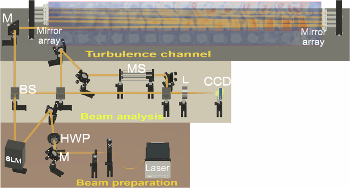
The setup is divided into three parts: beam preparation, turbulence channel, and beam analysis. Components included in diagram are mirrors (M), half wave plate (HWP), spatial light modulator (SLM), beam splitter (BS), mode sorter (MS), camera comprising charge-coupled device (CCD) for intensity measurements and Lenses (L).
SVM model based on optical intensity distribution
Images of the far-field intensity of the optical beam were recorded simultaneously along side the OAM spectra after propagation over the turbulent channel. As turbulence leads to random intensity fluctuations, the specific intensity shape recorded in any particular frame will vary uniquely and will not provide suitable data for accurate model training. Therefore, we process the 2D intensity to data, I(x, y) to record a distribution of power in along y-axis, I(y) of the image frame by considering the functions
and along the x-axis, I(x) considering the function
where N is number of pixels, where for our experimental data N = 160. As the turbulence distorts the optical field, the recorded intensity will be distributed over a larger area due to the additional spatial components induced by aberration, indicting a broader power spectral density function. Similar image processing is commonly used for the estimation of astronomic seeing, as it provides an estimate for the effective resolution of the optical system. We average I(x) recorded from each frame recorded over the same 3 s period used for the OAM spectra measurements. We train our SVM using the time averaged distributions of I(x) and I(y), where both arrays are concatenated into a 1D array of 320 elements. This array labeled in the same way as the OAM spectra data, and as with other presented data, verification data is from a different, independent data-set from the data used for training to assure accuracy in the presented results.
SVM model based on scintillation index
Utilizing the simultaneously recorded intensity information the scintillation index (SI) can be computed using the function
where I is the optical intensity and (leftlangle Irightrangle) denotes the ensemble average of the camera recorded intensity over the 3 s measurement window used for all data collection. The SI is labeled and trained using the an SVM model using the same procedure as both the OAM and intensity information to allow for direct comparison between the accuracy results.
Time Averaged OAM Spectrum Measurement
To measure the time-averaged OAM spectrum used for machine learning training, we record the intensity output from the mode sorter on a camera, as shown in Fig. 8a. The position along the x-axis of the camera output is directly related to the OAM content of the input optical beam63. Since OAM is an integer value, the output is binned, where all the pixel values are summed within each region (see Fig. 8b). Under the same turbulent strength, the specific distortion induced will vary over time, as depicted in Fig. 8a. Therefore, as we consider the ensemble average of the phase distortion for specific environmental conditions rather than the instantaneous distortion, it is important to record the time average of the OAM spectra over a 3 s measurement window (see Fig. 8c).
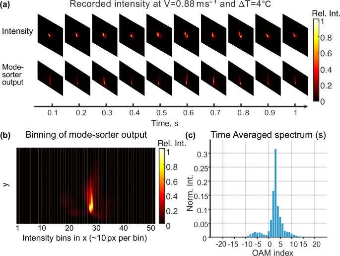
a Over time, the intensity output from the mode sorter is recorded by a camera. b Bin locations are allocated along the x-axis of the recorded image, where the received intensity is summed to measure the Orbital Angular Momentum (OAM) spectra. c Each bin corresponds to one OAM mode, and the intensity is subsequently normalized to the total intensity recorded across all measurement bins.
Greenwood frequency
The Greenwood frequency represents the necessary frequency or bandwidth for achieving the best correction with an adaptive optics system. It can be calculated with the equation (17)64,65
where λ represents the wavelength, θ signifies the zenith angle, V(z) stands for the wind-speed, and ({C}_{n}^{2}(z)) denotes the turbulence constant structure function. In our computation, θ is assumed to be 0. The turbulence constant structure function ({C}_{n}^{2}(z)) is determined from the scintillation of total energy at the receiving plane17. The scintillation index is computed over a duration exceeding 500 s, employing a 3 s averaging time window, as shown in Table 2). Figure 9 shows the measured Greenwood frequency for input OAM mode ℓ = 3 and wind speed of 2.23 ms−1.
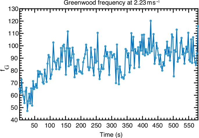
The input Orbital Angular Momentum (OAM) index is 3 and the averaging time is 3 s. The wind speed is 2.23 ms−1.


Responses