Yield gap decomposition: quantifying factors limiting soybean yield in Southern Africa

Introduction
Soybean (Glycine max (L.) Merril) is a legume crop that improves soil fertility1, human and animal nutrition2, and income3. The demand for soybeans continues to rise globally, while its production in Southern Africa is low, only contributing to 1% of the global output4. From this, commercial production dominates, and South Africa produces about 65% of the total regional produce, followed by Zambia, Malawi, and Zimbabwe5. Contribution by smallholder farmers (owning farms that are less or equal to 2 hectares6) is limited. This is attributed mostly to marginal profits due to low yields, in both quality and quantity, resulting from poor agronomic management practices, poor or low input use, poor soil fertility, inappropriate variety choices specific to agro-ecological zones, and erratic rainfall patterns and amounts7. Moreover, most governments in the region focus on staple food crops like maize8,9, leaving minimal support for the soybean value chain. Nonetheless, there is an increase in hectarage under soybean production.
Soybean production in Sub-Saharan Africa (SSA) is increasing as a result of hectarage under production5,10, but not yield increase per hectare. Undeniably, the increase in hectarage under soybean will continue11 and as observed from previous trends (from 2010 to 2020) (Omondi et al.5). This is driven by improved market prices12 as demand for soybeans as food and feed, especially in the poultry industry, rise13; diversification from maize14,15 particularly to enhance climate change adaptation and resilience16 and improve smallholder farmers’ nutrition17; improve soil fertility through biological nitrogen fixation18; break pest and disease cycles—pest control in integrated pest management such as fall armyworm and stemborer19,20 among others. Such land expansion for more production will gradually be unsustainable as the population grows; the land size per household reduces21,22 and hence yield per unit area requires improvement23. This yield increase per unit area could be realized by understanding the factors that contribute to the yield gap for specific agro-ecologies or individual farmers.
In the context of rainfed crops, yield gap is defined as the difference between the water-limited yield (Yw) and the actual yield (Ya) observed in farmers’ fields24. The water-limited yield (Yw) is defined as the maximum yield that can be obtained under rain-fed conditions in a specific biophysical environment without nutrient limitations or other yield reduction factors such as pests, diseases, weeds etcetera25. Therefore, yield gap decomposition enables portioning of each yield contributing factor7, for example, soil nutrient, seed rate, variety, weeds, diseases and pests etcetera to their respective yield gap value26. It thus strengthens targeting of specific interventions to specific agro-ecologies or farmers depending on their capability to implement such interventions or innovations i.e., if soybean variety is the most limiting, then it is given the primary priority, and more resources are deployed to narrow the yield gap.
Omondi et al.5 reported that the average soybean yield for Malawi in 2023 based on data from FAOSTAT was 39.8% lower while those of Zambia and Mozambique were 6.1% and 25.9% higher, respectively than Africa’s average yield in 2023. This indicates that the causes of yield gaps are country-specific and could further narrow to agro-ecologies, households, and individual farms. They also noted that in comparison to the global average yield, the yield gap widened in all three countries; the average soybean yield in the world was 195.2%, 99.0%, and 67.8% higher than in Malawi, Zambia, and Mozambique, respectively. Accordingly, they concluded that globally, some countries were narrowing their yield gaps and closer inching to the potential yield, while most countries in Sub-Sahara Africa lagged. They further compared FAOSTAT soybean yield in 2020 with the attainable soybean yield under breeding trials at the International Institute of Tropical (IITA) in those three countries and observed wide yield gaps for Malawi, Zambia, and Mozambique, respectively. This was even wider than the comparison with either Africa’s or the global average yield. Therefore, decomposing the yield gap i.e., identifying the causes of yield gaps in these countries and prioritizing interventions to narrow the gaps is necessary. Thus, this study assessed the contribution of various crop management practices and inputs to yield gap, the actual farmer-attainable soybean yield for each country, and the major factors limiting soybean productivity.
Results
Fertilizer application (quantity and type) to soybean plants was also a question posed to the farmers, only <5% responded positively, stating that they applied fertilizers. Owing to this low response, boundary line analysis of fertilizer effect on soybean yield wasn’t conducted in the three countries.
Despite the availability of some fertilizer blends for soybean in the market, for example, soya mix A or B (7-20-13 + S+Zn or 5-20-20 + S+Zn), many farmers in Malawi, Zambia, and Mozambique (approximately 95% of soybean farmers surveyed) do not apply fertilizer to legumes, including soybean.
Seed rate of soybean
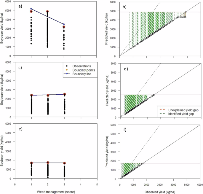
The soybean seed rate in Malawi ranged from 6.2 to 152.8 kg ha-1, however, the highest actual farmer yield (4882.7 kg ha-1) was obtained at 85.0 kg ha-1 (Fig. 1a, Table 1), and the yield gap was 27.3% (Fig. 2a, Table 1). The yield gap from 6.3% farms and upto 602.9 kg ha-1 grain yield couldn’t be explained by seed rate (Table 1) i.e., the data points that fell below the 1:1 line in the observed versus predicted yield graph (Fig. 1b). In Zambia, the lowest actual farmers’ seed rate was 19.6 kg ha-1 and the highest was 165.2 kg ha-1 producing 1049.5 kg ha-1 and 2500 kg ha-1 soybean grain yield, respectively (Fig. 1c, Table 1). This highest seed rate also produced the highest grain yield. The resulting yield gap was 58.0% (Fig. 2b), and the seed rate could explain 93.7% of this (Fig. 1d, Table 1). The actual farmers’ seed rate in Mozambique ranged from 14.2 to 293.5 kg ha-1 leading to 469.5 and 1299.0 kg ha-1 soybean grain yield, respectively (Fig. 1e, Table 1). However, 31.9 kg ha-1 produced the highest actual farmer grain yield of 1737.0 kg ha-1 in Mozambique. The yield gap between the highest actual farmer’s yield and the lowest was 63.8% (Fig. 1c), and in 8.9% of the farms, this yield gap could not be explained by the seed rate (Fig. 2f, Table 1) In comparing the other two countries with Malawi, which had the highest actual farmer yield, a 94.4% seed increase in Zambia still led to lower grain yield by 95.5%. Conversely, in Mozambique, the seed rate at which the highest grain was produced was lower than in Malawi (166.5% less), yet, soybean grain yield in Malawi was higher by 181.1%. Overall, the highest soybean yield gap resulting from seed rate was from Mozambique, followed by Zambia and then Malawi (Fig. 2 and Table 1). Additionally, yield gap from many farms in Mozambique compared to the other countries could not be explained by the seed rate.

a Study area showing the distribution of households in Malawi, Zambia, and Mozambique; b, c the average and maximum atmospheric temperature, respectively; d rainfall amount and e wind speed during the period during which the farmers reported soybean being in the field in various site.
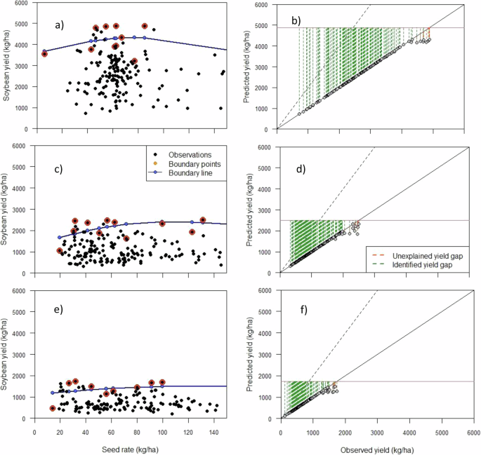
a, c, e Boundary lines and b, d, f yield gaps in Malawi, Zambia, and Mozambique, respectively. The 1:1 represents when the actual yield is equal to the predicted yield. The points that fall below the 1:1 line indicate yield gap that cannot be explained by the seed rate.
Soybean variety
The soybean varieties planted by the farmers in the three countries included: Tikolore, Makwacha, Nasoko, and Serenade in Malawi; Kafue (also called Tikolore in Malawi), Dina, Kamulanga (a local variety) in Zambia; Wamini (same variety as Tikolore and Kafue), Safari, and Serenade in Mozambique (Fig. 3). In Malawi, the highest actual farmers’ yield influenced by soybean variety was produced by Tikolore (4882.7 kg ha-1), whereas the lowest was produced by Nasoko (1710.4 kg ha-1) (Fig. 3a)—a yield gap of 64.9% (Fig. 6a and Table 1). This yield gap could be fully explained by the choice of soybean variety planted (Fig. 3b, Table 1). In Zambia, as in Malawi, Kafue variety (is Tikolore in Malawi) outperformed the rest, producing 2500 kg ha-1 against the lowest yield of 833.3 kg ha-1 from Kamulanga (Fig. 3c). This led to a 66.7% yield gap (Fig. 3b and Table 1), a yield gap that in 97.7% of the farms surveyed was attributed to the choice of soybean variety planted and 446.9 kg ha-1 grain yield could not be explained (Fig. 3d and Table 1). Interestingly, the same variety in both countries (Tikolore in Malawi or Kafue in Zambia) produced lower yields in Zambia compared to Malawi. Serenade produced higher yields (1660.4 kg ha-1) in Mozambique compared to all the other varieties, and Safari’s yield was the lowest (662.9 kg ha-1) (Fig. 3e) leading to a yield gap of 60.1% (Fig. 2c and Table 1). This yield gap could not be explained by the choice of soybean variety in 3.2% of the farms surveyed (Fig. 3f, Table 1). Altogether, the yield gap due to soybean variety was highest in Zambia, followed by Malawi, and then Mozambique (Table 1). Moreover, the yield gap that could not be attributed to the choice of soybean variety planted was also higher in Zambia compared to the other countries (Table 1).
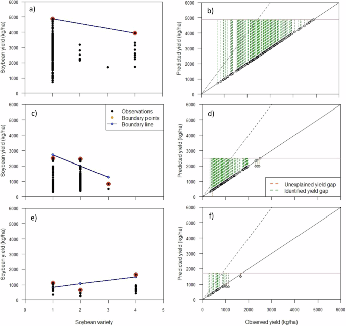
a, b represent boundary line and yield gap, respectively, in Malawi; similarly, c, d in Zambia; also, e, f in Mozambique. The names of the soybean varieties Malawi: 1—Tikolore, 2—Makwacha, 3—Nasoko, 4—Serenade; for Zambia: 1—Kafue (also called Tikolore in Malawi), 2—Dina, 3—Kamulanga (a local variety); for Mozambique: 1—Wamini, 2—Safari, 4—Serenade. The 1:1 represents when the actual yield is equal to the predicted yield. The points that fall below the 1:1 line indicate yield gap that cannot be explained by the soybean variety planted.
Disease damage
Disease damage was evaluated in the three countries using the scores: no sign of disease damage as ‘1’, ‘2’ as limited signs of disease damage, ‘3’ as moderate signs of disease damage, and ‘4’ as widespread signs of disease damage. In Malawi, the soybean farms with no signs of disease produced the highest yields (4848.3 kg ha-1), whereas the lowest was from farms with widespread signs of disease (1837.8 kg ha-1) (Fig. 4a) leading to a yield gap of 62.1% (Fig. 2a). Disease damage could not explain this yield gap in 4.6% of the farms and a grain yield of up to 542.2 kg ha-1 (Fig. 4b, Table 1). The highest soybean yield when there was no disease damage in Zambia was 2500 kg ha-1, while the farms with moderate signs of disease produced 1938.3 kg ha-1 (Fig. 4c). This caused a yield gap of 22.5% (Fig. 2b and Table 1). A yield gap that disease damage could explain well in 98.3% of the farms (Fig. 4d, Table 1). Similar to Malawi, farms with no signs of disease in Mozambique produced more soybean (1737.0 kg ha-1) than those with widespread disease (1314.9 kg ha-1) (Fig. 4d) leading to a yield gap of 24.3% (Fig. 2c and Table 1). However, in 1.9% of the farms, and up to 188.1 kg ha-1 of soybean grain of the yield gap could not be associated with disease damage (Fig. 4e). Overall, the yield gap attributed to disease damage, the number of farms and grain yield that could not be explained by disease damage was highest in Malawi (Fig. 2, Table 1).
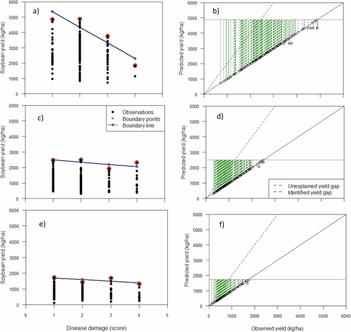
a The fitted boundary line, and b the yield gap associated with disease damage in Malawi; likewise for c, d in Zambia; equally for e, f in Mozambique. The scores for disease damage: 1—no sign of disease damage, 2—limited signs of disease damage, 3—moderate signs of disease damage, 4—widespread sign of disease damage. The 1:1 represents when the actual yield is equal to the predicted yield. The points that fall below the 1:1 line indicate yield gap that cannot be explained by disease damage.
Pest damage
In the three countries, pest damage was scored using a scale of ‘1’ as no sign of pest damage, ‘2’ as limited signs of pest damage, ‘3’ as moderate signs of pest damage, and ‘4’ represented widespread signs of pest damage. Like disease damage, yield after widespread pest damage in Malawi was 3005.4 kg ha-1 compared to lack of pest damage (4848.3 kg ha-1) (Fig. 5a) resulting in a yield gap of 38.4% (Fig. 2a and Table 1). This yield gap could not be explained by pest damage in 3.4% of the farms, similarly, the grain yield of up to 467.9 kg ha-1 (Fig. 5b, Table 1). In Zambia, soybean yields were highest in fields where there were no signs of pest damage and lowest where the pest damage was widespread (Fig. 5c). This led to a yield gap of 45.7% (Fig. 2b, Table 1) which could be explained by pest damage in 98.9% of the farms surveyed (Fig. 5d, Table 1). Maintaining pest-free soybean fields in Mozambique led to a higher yield of 1737.0 kg ha-1 in comparison to the lowest yields when the pest damage was widespread (Fig. 5e). The yield gap attributed to pest damage was 20.6% (Fig. 2c and Table 1), and those from 2.4% of the farms could not be explained by pest damage (Fig. 5f, Table 1). In general, pest damage led to higher yield reduction in Zambia, and yield gap from more farms could not be explained by pest damage (Fig. 2, Table 1).
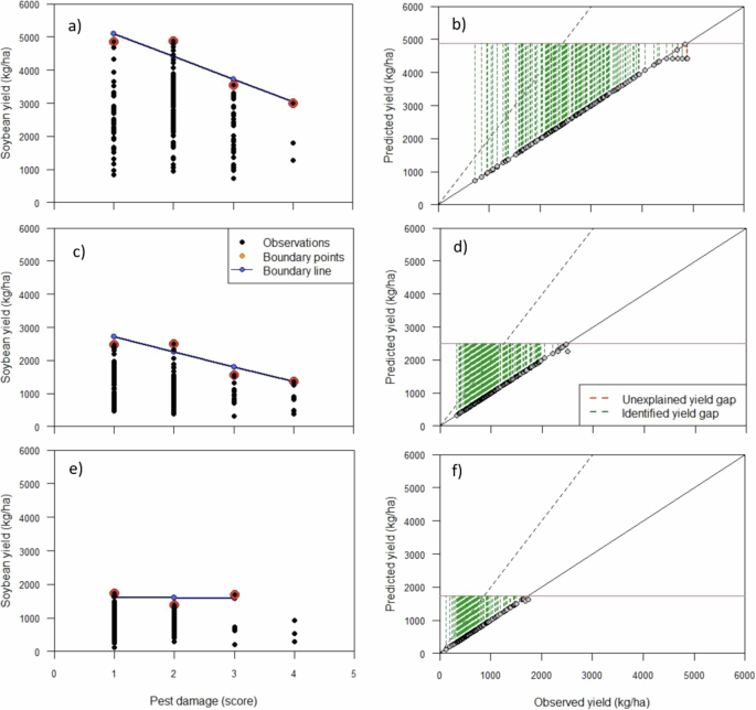
a The fitted boundary line and b the yield gap associated with pest damage of soybean in Malawi; similarly for c, d, respectively, in Zambia; also for e, f, respectively, in Mozambique. The scores for pest damage: 1—no sign of pest damage, 2—limited signs of pest damage, 3—moderate signs of pest damage, 4—widespread sign of pest damage. The 1:1 represents when the actual yield is equal to the predicted yield. The points that fall below the 1:1 line indicate yield gap that cannot be explained by pest damage.
Weed management
Weed management impact in the three countries was scored on a scale of ‘1’ representing well managed (no weed infestation), ‘2’ being moderately managed (some weeds observed), and ‘3’ as poorly managed (>half the field is infested with weeds). In the fields where there was no weed infestation in Malawi, soybean yield was highest compared (4882.7 kg ha-1) (Fig. 6a) to the lowest in highly weed-infested fields. This led to a yield gap of 34.9% (Fig. 2a and Table 1). This yield gap and up to 558.9 kg ha-1 could not be explained by weed infestation in 4.6% of the farms surveyed (Fig. 6b, Table 1). In Zambia and Mozambique, as in Malawi, well-weeded fields produced more soybean yield (Fig. 6), although the yield gaps due to weed infestation were negligible at 5.2% and 4.4% in Zambia (Fig. 2b and Table 1) and Mozambique (Fig. 7c and Table 1), respectively. Generally, weed infestation led to a higher yield gap in Malawi(Fig. 2), although, compared to Zambia and Mozambique yield gap from many farms could not be explained by weed infestation and more farms (Table 1).
a, c, e The fitted boundary line, and b, d, f the yield gap arising due to weed management in Malawi, Zambia, and Mozambique, respectively. The scores for weed management: 1—well managed (no weed infestation), 2—moderately managed (some weeds observed), 3—poorly managed (>half the field is infested with weeds). The 1:1 represents when the actual yield is equal to the predicted yield. The points that fall below the 1:1 line indicate yield gap that cannot be explained by weed infestation.
Discussion
Reaching potential yield is always hindered by various factors5,7,27. Identifying the most yield-limiting factors could lead to prioritization of interventions and targeted approaches to increase yields from actual to attainable to potential per unit area. Through yield gap decomposition using boundary line analysis, this study has identified the limiting factors for soybean yield increase in Malawi, Zambia, and Mozambique. Furthermore, when using boundary line analysis it is possible to check if one of the factors affecting yield in a given location can explain the identified yield gap28—this has been done in this study. This not only boosts prioritization of interventions but also enhances targeting.
Soybean variety is the most yield-limiting factor in both Malawi and Zambia and in Malawi it largely explains the yield gap observed. Interestingly, the popular soybean variety that performs better in both countries is the same (Tikolore in Malawi or Kafue in Zambia or Wamini in Mozambique also called TGx 1740‐2 F)—an improved promiscuous variety29,30. Abate, (2012) observed that improved varieties (e.g., TGx 1740‐2 F in Malawi) had a yield advantage of 38% over local check, and the results, especially from Zambia attest to this, since the local variety (Kamulanga) performed dismally. In as much as the improved variety that performed better in both Zambia and Malawi were similar, there yield gaps with the least performing varieties were variable. The difference in varietal yields in both environments is mostly due to the differences in agro-ecologies—at Katete and Sinda in Zambia, the rainfall was 1004.5 mm and 811.2 mm, respectively whereas at Kasungu and Lilongwe, the rainfall was 1854. 4 mm and 1022.5 mm, respectively during the growth period (Fig. 7). This high amount of rainfall in Malawi sites provided the required soil moisture to drive the observed yields since soybean’s optimal water requirement is between 400 and 700 mm under rainfed31. Additionally, the soils in Kasungu could be rich in phosphorus compared to Katete and Sinda, and P is key for soybean yield improvement32,33. Despite better soil water and nutrient conditions in Malawi for the soybean variety, Tikolore, the least performing variety that led to the higher yield gap probably had lower nutrient conversion efficiency. Indeed34, confirms that varieties with low nutrient conversion efficiency can have dismal performance even under suitable nutrient conditions. Disease damage is the second most limiting factor in Malawi, even though it could not explain up to 542.2 kg ha-1 grain yield of the yield gap. Disease damage is the second most limiting factor in Malawi because in 2022/2023 season when the survey was conducted there was a wide outbreak of soybean rust in most of the Southern African countries4,35. It was devastating in Malawi35 as most farmers were unable to control the disease in time mainly because they assumed the crop was approaching physiological maturity (feedback during the survey). Certainly, they had poor knowledge to identify soybean rust symptoms, cemented by Murithi et al.4. Indeed, soybean rust symptoms can easily be confused with brown spots or bacteria pustules36, and over time with physiological maturity, and hence it requires seasoned skills and knowledge to identify. Despite this, there is a general recommendation in the region to soybean farmers to always apply fungicide at the beginning of flowering, and then at two to three weeks intervals depending on its severity in the area37. A recommendation that perhaps was observed more by farmers in Zambia, where the disease damage was minimal, compared to those in Malawi because of large-scale production in Zambia5 hence more investment in production such as mechanization38 or application of chemicals39. Besides, poor skills to identify soybean rust, and lack of early control40, high wind current41, high rainfall amount42, and humidity43 probably contributed to vast spread and attacks of the rust in Malawi. This was the case in Malawi compared to other agro-ecologies (Zambia and Mozambique), as the wind speed in Kasungu and Lilongwe were above the other sites (Fig. 7) which encouraged dispersion of the rust spores41, coupled with high rainfall amounts (as in Fig. 7), improved the attachment and development of the spores36. Moreover, the high yield gap under weed management indicates that weed pressure in Malawi was high, further increasing the host availability for rust—serving as an alternative host44, and increasing competition for resources such as nutrients45, thus reducing the crop vigour. It is only in Zambia where the pest damage led higher yield gap than disease damage, possibly due to the variety mostly grown by the farmers (Kafue) wasn’t susceptible to pests as the local variety (Kamulanga). Additionally, most Zambian soybean farmers sometimes intercrop soybean with sunflower, thus offering more food to pests, like Dectes texanus46 and Chrysodeixis includens47, increasing their fecundity and population.
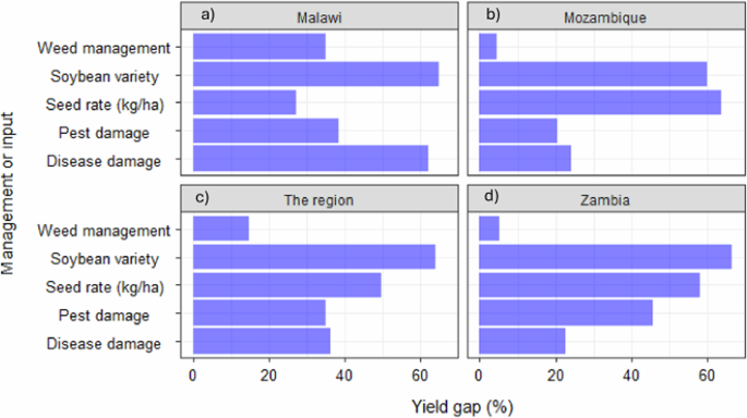
In a Malawi, b Mozambique, c Zambia, and d in all the three countries (Malawi, Zambia, and Mozambique).
While in both Malawi and Zambia, soybean variety contributed to the highest yield gap, seed rate was the highest contributor in Mozambique despite it not being to explain up to 457.4 kg ha-1 grain yield of the yield gap. Remarkably, the results indicated that in Mozambique, the minimum and maximum seed rates were higher than the other two countries, an indication that a higher seed rate could lead to diminishing returns i.e., higher plant population, thus competition for resources such as light and nutrients48,49,50. Undeniably, Silva et al.51 observed that a higher plant population increases competition for resources hence reducing yields. Strengthening this is the planting arrangement and spacing of 50 cm by 10 cm in Mozambique52 compared to the other countries, for example, in Malawi farmers prepare ridges spaced at 75 cm apart and on each they make two grooves (20–30 cm apart) to plant soybeans53. This minimizes competition among the plants. Additionally, the seed rate recommendation in Malawi and Zambia by the government is 60–65 kg ha-1 53 and 80-110 kg ha-1 depending on the variety54, respectively compared to 50–60 kg ha-1 in Mozambique. Moreover, the seed viability in Mozambique could be low due to the recycling of previously certified seed, a question that wasn’t clearly elaborated in the survey questionnaire. Malita et al.55 confirmed that most farmers regularly recycle legume seeds which leads to a decline in viability56 causing repeated gapping and hence higher seed rate. This probably occurred in Mozambique due to poor soil nutrients or moisture57, a scenario corroborated by early planting with minimum soil moisture and low application of fertilizers58, especially phosphorus to soybean59—also supported by the survey results of this study in which only a few farmers apply fertilizer to soybeans.
Across the Southern Africa region (Malawi, Zambia, and Mozambique), besides soil fertility and fertilizer application which was not determined in this survey, soybean variety causes a higher yield gap, followed by the seed rate, and then disease damage, especially soybean rust4. Despite breeding efforts and the release of promiscuous varieties i.e., the Tropical glycine cross (TGx) lines from the International Institute of Tropical Agriculture29 and other seed companies, the soybean seed system is still plagued by many problems. Mainly the price of certified improved seeds is high so most farmers can’t afford them, lack of clear distribution channels and knowledge of suitable site-specific varieties60. Interestingly from the results of this study, some countries have higher seed rates than the government recommendation. An indication of availability of seed, but most likely recycled seed that has low viability which requires a high seed rate to obtain the desired plant population. Indeed recycled seeds have reduced viability56,61.
Minimizing yield gap is key to increasing yield per unit area and agronomic gain, however, it is necessary to understand the yield-limiting factors and prioritize interventions considering the few resources that smallholder farmers have. This study has shown that to close the soybean yield gap, besides soil nutrients, soybean variety is the most limiting factor in Malawi and Zambia followed by disease damage in Malawi and seed rate in Zambia. Whereas, in Mozambique, seed rate is significant, although the seeds should have high viability, followed by the variety. Overall, in the Southern Africa region (Malawi, Zambia, and Mozambique) the major soybean yield gap contributors are: variety, seed rate, and disease damage, especially soybean rust, in that order.
Release of improved high-yielding promiscuous soybean varieties like Chitedze 4 and Tikolore in Malawi, Wamini and Kafue in Mozambique and Zambia, respectively, notwithstanding, most farmers are yet to adopt suitable varieties for their specific regions. And even those who have adopted them tend to recycle the seeds leading low growth vigour and poor yields. Thus, there is need to improve certified seeds production through the community-based seed producers, enhance its access and availability and quality monitoring – essentially strengthening the soybean seed production system with a focus on the end-user benefits. Secondly, and linked to the seed systems, seed rate is mostly lower due to recycling and poor germination, which can be addressed by strengthening the seed system, ensuring appropriate planting time adhering to effective soil moisture, and suitable planting population. Thirdly, disease surveillance needs strengthening, with the spread and help of smartphones and feature phones, farmers self-reporting of disease outbreaks like soybean rust could be tracked via social media, and real-time solutions offered to prevent further yield losses.
Methods
Sites
The data was collected in two districts of Malawi (Lilongwe and Kasungu) from farmers located between 12.82°-13.97° S and 33.44°-33.74° E; in Zambia in Chipata and Sinda districts (14.21°-14.20° S and 31.85°-32.22° E), and in Mozambique in Angonia district (14.67°-14.73° S and 33.96°-34.38° E) in 2023. These areas are at an altitude of 915–1557 m above sea level, with the region predominantly referred to as the Chinyanja Triangle (Fig. 7a). In this region, the average and maximum atmospheric temperature, rainfall amount, and wind speed from 1st October 2022 to 30th April 2023, the period during which most of the farmers reported soybean being in the field (from planting to harvesting) is presented in Fig. 7b–e. This area is within the Zambezi River Basin and lies between the Luangwa River on the West, Lake Malawi, and River Shire on the East, and Zambezi river on the South. It is popular with the Chichewa/Chinyanja-speaking people sharing a similar history, language, and culture across the Eastern province of Zambia, the Central regions of Malawi, and the Tete Province of Mozambique. The three communities in the three countries are differentiated by biophysical conditions, as well as country-specific political and economic conditions. The Chinyanja Triangle is dominated by maize-based farming systems.
Data collection and crop cut survey
Crop cut surveys generate production data through direct measurement and it is widely used as a method of yield estimation. The major objective of a crop-cut survey is to measure actual crop yields under actual farmer management conditions through randomly selected sample plots within a crop field. From the selected plot, a sub‐plot is harvested and weighed appropriately. Then, the yield per unit area is calculated as the weight of the harvested crop yield adjusted for grain moisture content62.
The yield cut survey was conducted in Malawi, Zambia, and Mozambique following the protocol by CIMMYT (2023). In each country, 180 farmers/households growing soybeans (Fig. 7) responded to the survey questions which were administered by trained enumerators in a standardized questionnaire through ODK63 and uploaded on ONA64. In Malawi, data was collected from 120 households in Kasungu and 60 households in Lilongwe districts, whereas in Zambia 120 households were from Katete and 60 from Sinda districts. In Mozambique, all the 180 households were from Angonia district. The survey questions were on administrative levels, farmer name and gender, location, land size, crop grown and management practices (weeding, pest and disease control), actual yield cut for yield calculation, inputs, inputs and produce prices.
Disease damage was evaluated in the three countries by scoring: no sign of disease damage as ‘1’, ‘2’ as limited signs of disease damage, ‘3’ as moderate signs of disease damage, and ‘4’ as a widespread sign of disease damage. In the three countries, pest damage was scored using a scale of ‘1’ as no sign of pest damage, ‘2’ as limited signs of pest damage, ‘3’ as moderate signs of pest damage, and ‘4’ represented widespread signs of pest damage. Weed management impact in the three countries was scored on a scale of ‘1’ representing well managed (no weed infestation), ‘2’ being moderately managed (some weeds observed), and ‘3’ as poorly managed (>half the field is infested with weeds).
In the yield cut protocol62, GPS coordinates, and area measurements were embedded in the ODK tool as part of the survey. The farmers were registered with unique farm identifiers (IDs) for each field and their plot areas were measured using the polygon option by walking around the perimeter of the plot. The field was then divided into four quadrants assuming that it was a rectangle. This was followed by assuming a diagonal line from the northwest (NW) to the southeast corners (SE) placing three sub-plots of 2 m by 2 m where the actual crop cut was to be conducted, the first on the top left quadrant, the second at the center, and the last on the bottom right. After this, the above-ground part of soybean was cut within each 2 m by 2 m sub-plot, the pods were separated from the haulms, threshed and the grains weighed. The fresh weight of the grains was recorded and later dry weight to 12% moisture content. The dry weights were used to calculate the yield per hectare for each field/farmer by averaging the three 2 m by 2 m sub-plots.
Yield gap decomposition using boundary line analysis
In the boundary line analysis (BLA), the water-limited yield (Yw) is derived from the highest farmers’ yield which is defined as the average top 10% of farmers’ yields whereas the remaining 90% forms the actual farmers’ yields (Ya) that can be achieved for a given input level in a well-defined biophysical environment.
Various parameters were collected during the survey, however, those subjected to boundary line analysis were yield (kg ha-1), seed rate (kg ha-1), soybean variety, disease and pest damage, and weed management.
The continuous variables such as seed rate were analysed, whereas the categorical variables/management variables such as weed management, disease and pest damage, and variety type were first given numerical codes before analysis.
Even though there are no generally agreed protocols for BLA, Hajjarpoor et al.65 outlined the following important processes:
-
1.
Examining the scatter plot of data: a scatter plot (XY chart) should be prepared with crop yield as the dependent variable and one selected independent variable (e.g., weeding).
-
2.
Removal of the outliers.
-
3.
Selection of the data points from the upper limit of the data for curve fitting.
-
4.
Fitting a function to the data points in 2.
The above processes were conducted in R66. The R packages installed and loaded included for the analysis included “splines”, “metrics”, “dplyr”, “tidyr”, “knitr”, “reshape2”, “ggplot2”, “mass”, “ggstatsplot”. After data was uploaded and boxplot analysis was conducted to identify outliers and eliminate them, boundary line models are susceptible to the effects of outliers65. The boundary line (BL) point function was defined, and the ‘X’ variable of interest—selected dry grain yield of soybean in our case. Using the binning approach, which is a heuristic approach, the ‘X’ variables were split into ten quantiles (from 0.1 to 1.0), and BL points for each quantile were defined based on maximum value or on the yields when approaching the 95th quantile. The highest farmers’ yields were set at the average of top 10% of the actual farmers’ yields to represent the Yw while the rest were Ya for every site i.e., each site was treated individually assuming that its biophysical characteristics are unique to itself, for example, the values for Kasungu in Malawi were calculated individually and not combined with those from either Angonia in Mozambique or Katete in Zambia. This was to ensure that yields within a given agro-ecology are treated the same and no introduction of variability due to biophysical differences from other regions. After setting the boundary points, the ‘Y’ variables were defined, and yield decomposition analysis was performed for each variable. The boundary line was fitted: for the continuous variables like seed rate and the discrete variables like disease damage in this study, Gaussian General Linear Model and Poisson General Linear Model were used, respectively. The results were then plotted as yield gap indicating the boundary points and the boundary line. Followed by the determination and the plotting of the identified yield gap (IYG), and unexplained yield gap (UYG). The yield gap estimation and decomposition were conducted by plotting the predicted yield (estimated using the boundary lines) against the actual yields. The continuous red line on each observed versus predicted yield graph represents the highest yield observed in the study area and it is taken as the attainable yield. The 1:1 line represents the situation when the actual yield is equal to the predicted yield. The points that fall below the 1:1 line indicate the unexplained yield gap i.e., the yield difference between the predicted and attainable yield that can not be explained by the most limiting factor.
After fitting the boundary lines, the percent yield gap for each site was calculated as follows:


Responses